

Infrared (IR) meibography is an imaging technique to capture the Meibomian glands in the eyelids. These ocular surface structures are responsible for producing the lipid layer of the tear film which helps to reduce tear evaporation. In a normal healthy eye, the glands have similar morphological features in terms of spatial width, in-plane elongation, length. On the other hand, eyes with Meibomian gland dysfunction show visible structural irregularities that help in the diagnosis and prognosis of the disease. However, currently there is no universally accepted algorithm for detection of these image features which will be clinically useful. We aim to develop a method of automated gland segmentation which allows images to be classified.
MethodsA set of 131 meibography images were acquired from patients from the Singapore National Eye Center. We used a method of automated gland segmentation using Gabor wavelets. Features of the imaged glands including orientation, width, length and curvature were extracted and the IR images enhanced. The images were classified as ‘healthy’, ‘intermediate’ or ‘unhealthy’, through the use of a support vector machine classifier (SVM). Half the images were used for training the SVM and the other half for validation. Independently of this procedure, the meibographs were classified by an expert clinician into the same 3 grades.
ResultsThe algorithm correctly detected 94% and 98% of mid-line pixels of gland and inter-gland regions, respectively, on healthy images. On intermediate images, correct detection rates of 92% and 97% of mid-line pixels of gland and inter-gland regions were achieved respectively. The true positive rate of detecting healthy images was 86%, and for intermediate images, 74%. The corresponding false positive rates were 15% and 31% respectively. Using the SVM, the proposed method has 88% accuracy in classifying images into the 3 classes. The classification of images into healthy and unhealthy classes achieved a 100% accuracy, but 7/38 intermediate images were incorrectly classified.
ConclusionsThis technique of image analysis in meibography can help clinicians to interpret the degree of gland destruction in patients with dry eye and meibomian gland dysfunction.
La meibografía de infrarrojos (IR) es una técnica de imagen que capta las glándulas de Meibomio de los párpados. Dichas estructuras de la superficie ocular son responsables de la producción de la capa lipídica de la película lagrimal, que ayuda a reducir la evaporación de las lágrimas. En un ojo sano normal, las glándulas tienen características morfológicas similares en términos de anchura espacial, elongación en plano y longitud. Por otro lado, los ojos con disfunción de las glándulas de Meibomio muestran irregularidades estructurales visibles que ayudan al diagnóstico y pronóstico de la enfermedad. Sin embargo, actualmente no existe un algoritmo universalmente aceptado para la detección de dichas características de imagen que sea clínicamente útil. Nuestro objetivo es desarrollar un método de segmentación automatizada de la glándula que permita la clasificación de las imágenes.
MétodosSe adquirió una serie de 131 imágenes meibográficas procedentes de los pacientes del Centro Ocular Nacional de Singapur. Utilizamos un método de segmentación automatizada de las glándulas, mediante ondículas de Gabor. Se extrajeron las características de las imágenes de las glándulas tales como orientación, anchura y curvatura, realzándose las imágenes de IR. Se clasificaron las imágenes como “sanas”, “intermedias” o “insanas”, mediante el uso de una máquina clasificadora de vectores de soporte (SVM). La mitad de las imágenes se utilizaron para probar la SVM y la otra mitad para validación. Independientemente de este procedimiento, las meibografías fueron clasificadas por un médico clínico experto, con arreglo a las 3 categorías anteriores.
ResultadosEl algoritmo detectó correctamente el 94% y el 98% de los píxeles de la línea media de la glándula y de las regiones inter-glandulares, respectivamente, en las imágenes sanas. En las imágenes intermedias, se obtuvieron porcentajes correctos de detección del 92% y 97% de los píxeles de la línea media de la glándula y de las regiones inter-glandulares, respectivamente. El porcentaje positivo y cierto de detección de las imágenes sanas fue del 86%, y del 74% para las imágenes intermedias. Los correspondientes porcentajes de falsos positivos fueron del 15% y 31%, respectivamente. Utilizando la SVM el método propuesto logró un 88% de precisión en la clasificación de imágenes conforme a las 3 categorías. La clasificación de las imágenes de las categorías sana e insana logró un 100% de precisión, aunque 7/38 de las imágenes intermedias fueron clasificadas incorrectamente.
ConclusionesEsta técnica de análisis de imágenes en la meibografía puede ayudar a los médicos clínicos a interpretar el grado de destrucción de una glándula en pacientes con ojo seco y disfunción de la glándula de Meibomio.
Clinical research on dry eye syndrome is currently receiving much attention.1–12 In particular, in the study of meibomian gland dysfunction, which is a major cause of dry eye,1 gland dysfunction can be diagnosed by directly observing the morphology of the meibomian glands using meibography. Recently, a non-contact, patient-friendly infrared meibography method was developed that is fast and greatly reduced the discomfort to the patient.8–10 This advance allows meibography to be used routinely in clinical research.
When analyzing meibography images, it is important to quantify the area of meibomian gland loss. Grades are then assigned to the image based on the area of gland loss, which in turn serve as an indicator of meibomian gland dysfunction. The loss of meibomian glands in the upper and lower eyelids have been studied.8,4,11,12 The subjective and objective grading of meibography images have also been assessed,7 and it has benn also demonstrated that precise calculation of the area of meibomian gland loss using a computer software can lead to greatly improved repeatability in the application of grading scales.4–6 In addition, other meibomian gland features such as the width and tortuosity of the glands can be accurately computed and analyzed. Srinivasan et al. 11 have also reported similar progress. These recent works demonstrated the advantages of a computerized approach to analyzing meibomian glands in meibography images.
In these recent works on computerized classification of meibomian gland loss, the images were analyzed using the image editing software ImageJ. The user needs to be involved, such as identifying the gland region on the image. In other words, the user needs to tell the software where the glands are. If a large number of images is involved, this process is tedious and time consuming. Also, different users may draw the gland region differently, leading to inter-observer variability. It would be more efficient if the glands can be analyzed automatically without any input from the user. This way, the results and conclusions of the analysis will not depend on any particular clinical examiner, and is also much faster and less laborious, making it useful when a large population is involved in a clinical study. Koh et al. 12 introduced the first attempt toward this goal. Image features such as gland lengths and widths are used together with a linear classifier to accurately differentiate between healthy and unhealthy meibography images. A series of heuristic image processing methods are applied to detect the gland and inter-gland regions’ mid-lines which are further used to estimate gland widths and lengths. The method can only differentiate between healthy and unhealthy meibography images. Intermediate stages of the syndrome can not be identified.
Further improvement in automated diagnosis requires precise gland and inter-gland segmentation. The gland and inter-gland boundaries as well as their mid-lines should be detected precisely for further performance improvement in automated assessment. Thus, the aim of this paper is to develop algorithms that can detect meibomian glands in meibography images without user input, and enhance the input IR images so that it becomes visually easier to assess Meibomian gland structures. Furthermore, the detected gland and inter-gland midlines are used to extract features. Different than Koh et al. 12, these features are used together with support vector machiene (SVM) classifier to achieve three level of classification: “healthy”, “intermediate” and “unhealthy”. To the best of authors knowledge, it is the first time that meibography images are used to assess three-level gradation.
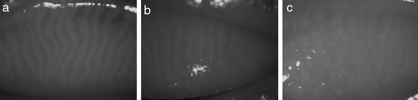
MethodologyAs shown in Fig. 1, the captured IR images of the inner eyelids have several features that makes it challenging to automatically detect the gland regions: (1) low-contrast between gland and non-gland regions, (2) specular reflections caused from smooth and wet surfaces, (3) inhomogeneous gray-level distributions over regions because of thermal imaging, (4) non-uniform illumination, and (5) irregularities in imaged regions of ocular surface.
 healthy, (b) intermediate, and (c) unhealthy.")
Even though there are diversities in imaging conditions, the gland regions have higher reflectance with respect to non-gland regions. Thus, the image regions corresponding to glandular structures have relatively higher brightness with respect to neighbouring non-gland regions. However, because of the above mentioned imaging conditions, the conventional methods such as local thresholding is not suitable for partitioning the image into gland, inter-gland and non-gland regions. Thus, a local filtering approach is employed. Gabor filtering is utilized as local filtering due to its parametrization in shape, local spatial support, and orientation.
Gabor FilteringThe family of two-dimensional (2D) Gabor filters can be used to model the spatial summation properties of simple cells.13 A modified parametrization of Gabor functions is used to take into account restrictions found in experimental data.14,15 The following family of 2D Gabor functions are employed to model the spatial summation properties of simple cells15:
where Gα(x,y)∈ℝ,(x,y)∈Ω⊃ℝ2 is Gabor function, the arguments x and y specify the position of a light impulse in the visual field and α={xc, yc, σ, γ, λ, θ, ψ} is parameter set which is defined as follows.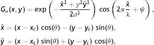
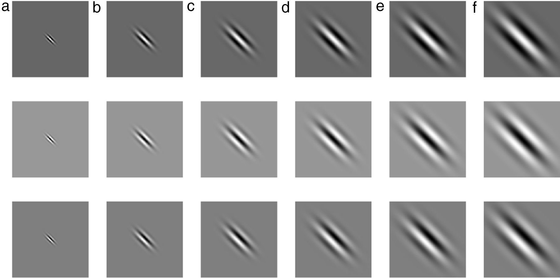
The pair (xc, yc)∈Ω specifies the center of a receptive field in image coordinates, meanwhile the size of the receptive field is determined by the standard deviation σ of the Gaussian factor. The parameter γ∈(0.23, 0.92)14 which is called the spatial aspect ratio, determines the ellipticity of the receptive field. The parameter λ is the wavelength and 1/λ is the spatial frequency of the cosine factor. The ratio σ/λ determines the spatial frequency bandwidth, and, therefore, the number of parallel excitatory and inhibitory stripe zones which can be observed in the receptive field as shown in Fig. 2. The half-response spatial frequency bandwidth b∈[0.5, 2.5] (in octaves)14 of a linear filter with an impulse response according to Eq. (1) is the following function of the ratio σ/λ14:
or inverselyThe angle parameter θ∈[0, π) determines the orientation of the normal to the parallel excitatory and inhibitory stripe zones which is the preferred orientation from the y-axis in counterclockwise direction. The parameter ψ∈(−π, π] is a phase offset that determines the symmetry of Gα(x, y) with respect to the origin: for ψ=0 and ψ=π it is symmetric (or even), and for ψ=−π/2 and ψ=π/2 it is antisymmetric (or odd); all other cases are asymmetric mixtures.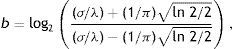
=(0, 0), γ=0.5, b=1.0 octave (σ/λ=0.56), θ=π/4, ψ=0 (first row), ψ=π (second row), ψ=π/2 (third row) and (a) λ=10 pixels, (b) λ=20 pixels, (c) λ=30 pixels, (d) λ=40 pixels, (e) λ=50 pixels, and (f) λ=60 pixels on 256×256 pixels grid, which model the receptive field profile of a simple visual cell. Gray levels which are lighter and darker than the background indicate zones in which the function takes positive and negative values, respectively.")
Normalized intensity map of Gabor functions with parameters (xc, yc)=(0, 0), γ=0.5, b=1.0 octave (σ/λ=0.56), θ=π/4, ψ=0 (first row), ψ=π (second row), ψ=π/2 (third row) and (a) λ=10 pixels, (b) λ=20 pixels, (c) λ=30 pixels, (d) λ=40 pixels, (e) λ=50 pixels, and (f) λ=60 pixels on 256×256 pixels grid, which model the receptive field profile of a simple visual cell. Gray levels which are lighter and darker than the background indicate zones in which the function takes positive and negative values, respectively.
In this work, without loosing of generality, it is assumed that Gabor function is centred at the coordinate plane of the receptive field, i.e., (xc, yc)=(0, 0), spatial aspect ratio is γ=0.5, b=1.0 octave (σ/λ=0.56). Since σ/λ=0.56 is constant, one of the variables σ or λ is dependent to other. It is assumed that λ is independent to fine tune the spatial frequency characteristics of Gabor function. Thus the parameter σ is not used to index the receptive field function;
It is worth to note that the 2D Gabor function Gα has a bias term (or DC term), i.e.,
The DC term is subtracted from Gα to remove the bias, i.e.,and the resultant Gabor filter is normalized by square root of its energy as
Using the above parametrization for 2D Gabor function, one can compute response Iα to an input 2D image I as
where “*” is 2D convolution operator. Eq. (7) can be efficiently computed in Fourier transform (F) domain, i.e., Iα=F−1(F(I)F(Gα)) where F−1 is the inverse Fourier transform.Feature Extraction and Gland Detection
In IR images, gland and inter-gland regions form ridges and valleys, respectively. One can easily notice that realizations of Gabor functions shown in the first row of Fig. 2 for ψ=0.0 can be used to model the local structure of gland which is surrounded by inter-gland regions. The white main lobe in the middle represents the gland, and the black side lobes on both sides of the main lobe represent inter-gland regions. The parameter λ can be used as an estimate for the spatial width, and the parameter θ can be used as an estimate to local orientation of sub-gland structure. Similarly, for ψ=π the Gabor functions shown in the second row of Fig. 2 can be used to detect the regions between two glands, i.e., the black lobe in the middle represents the inter-gland region, and the white side lobes on both sides of the main lobes respresent gland regions. The third row row of Fig. 2 shows Gabor functions for ψ=π/2 which are good representation of edges. Thus, gland and inter-gland regions are obtained using variants of filters shown Fig. 2. Let Iλ,θ+, Iλ,θ− and Iλ,θe are defined as Iλ,θ+=Iα+, Iλ,θ−=Iα− and Iλ,θe=Iαe where α+={xc=0, yc=0, σ, γ=0.5, λ, θ, ψ=0}, α−={xc=0, yc=0, σ, γ=0.5, λ, θ, ψ=π}, αe={xc=0, yc=0, σ, γ=0.5, λ, θ, ψ=π/2}. The response image Iλ,θ+ is expected to have high response on gland regions, meanwhile, Iλ,θ− produces high response on inter-gland regions. The response image Iλ,θe is expected to produce high response on boundaries or edges. Note that Iλ,θ+=−Iλ,θ−, thus, only Iλ,θ+ is computed and on the response image, positive and negative response values of Iλ,θ+ are referring to gland and inter-gland regions, respectively.
In order to achieve local gland and inter-gland representation using Gabor functions, one needs to make a correct estimation for λ and θ for local structure width and orientation, respectively. The parameter λ takes discrete integer values from a finite set {λi} and can be estimated according to expected spatial width of the consecutive gland and inter-gland regions. Meanwhile, it is expected that sub-gland structure can have any orientation in between [−π/2, π/2). However, it is impractical to test every possible orientation. Thus, the parameter θ is discritized according
where Nθ is the total number of discrete orientations.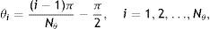
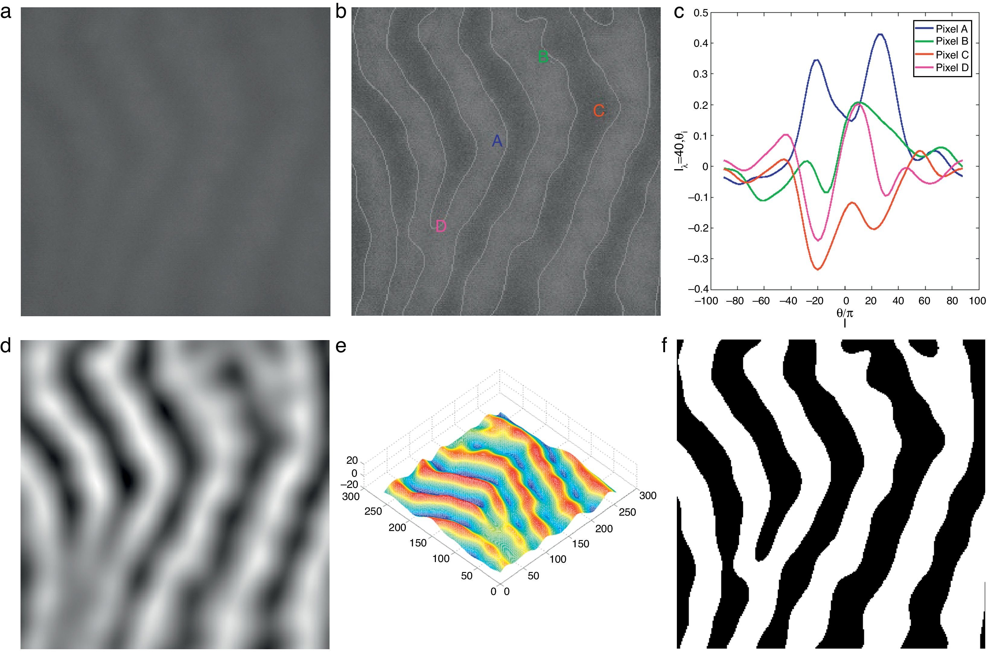
The main motivation of using Gabor filters for gland and inter-gland structure detection is due to the reason that local structures of gland and inter-gland regions can be represented by a proper Gabor filter. The width and elongation of the local structure is estimated by the wavelength λ and orientation θ of the filter. Thus, for a correct estimation of λ and θ for each pixel, Gabor filter response is positive over gland region, meanwhile it is negative over inter-gland regions. In order to demonstrate, a sub-region of IR image from Fig. 1(a) is used, and Gabor filter responses on different pixel locations falling into regions of gland and inter-gland regions are shown in Fig. 3(c) for a fixed λ and variable θ. Pixels A and B are on gland regions, and pixel C is on inter-gland region. The maximum of absolute valued Gabor filter responses of pixels A and B are realized when the sign of Gabor filter response is positive (+), while, the sign of the maximum value of absolute valued Gabor filter response is negative (−) for pixel C. For a pixel a gland region which is surrounded by non-gland regions, there is a high difference between magnitudes of positive maximum and negative minimum. Similarly, for a pixel over inter-gland region which is surrounded by gland regions, there is a high difference between magnitudes of negative minimum and positive maximum. However, when the pixel resides on a region which has very close proximity to both gland and inter-gland regions, e.g., pixel D on Fig. 3(b), the difference between magnitudes of positive maximum and negative minimum is small as shown in Fig. 3(c). It is also clear that the sign of average Gabor response is (+) over gland regions, and is (−) over inter-gland regions.
 input 256×256 pixels IR image cropped from Fig. 1(a); (b) contrast enhanced IR image on which the boundary pixels detected from binary image in (f) is overlayed and corresponding pixel locations over which Gabor filter responses are observed; (c) Gabor filter responses of pixels shown in (b); (d) average Gabor filter response Iλ=40 of (a) computed according to Eq. (10); (e) surface plot of (d); (f) binarized Gabor filter response Bλ according to Eq. (11). (For interpretation of color in the artwork, the reader is referred to the web version of the article.)")
Demonstration of Gabor filter responses over different spatial locations for λ=40 pixels and Nθ=72: (a) input 256×256 pixels IR image cropped from Fig. 1(a); (b) contrast enhanced IR image on which the boundary pixels detected from binary image in (f) is overlayed and corresponding pixel locations over which Gabor filter responses are observed; (c) Gabor filter responses of pixels shown in (b); (d) average Gabor filter response Iλ=40 of (a) computed according to Eq. (10); (e) surface plot of (d); (f) binarized Gabor filter response Bλ according to Eq. (11). (For interpretation of color in the artwork, the reader is referred to the web version of the article.)
Thus for a given λ, the mean Gabor response Iλ is computed as follows:
which is approximated asIn the above equation, the denominator represents the average edge energy along the orthogonal direction to the main filter used to detect the local structures.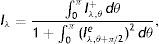
In Fig. 3(d) the average Gabor filter response to an input image in Fig. 3(a) is shown for λ=40 pixels and Nθ=72. The corresponding surface plot is given in Fig. 3(e). It is clear from Fig. 3(d) and (e) that the filter gives high positive responses on gland regions, meanwhile, it produces low negative responses on non-gland regions. Thus using this observation, one can easily segment out gland regions from inter-gland regions using the sign of filter response, i.e.,
where H(a)∈{0, 1} is a binary function defined as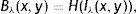
In Fig. 3(f) the binarized Gabor filter response according to Eq. (11) is shown. Overall, the segmentation result looks satisfactory. However, it can be observed that at pixel D two glands regions are merging together where the separation between two glands is distinct in surface plot shown in Fig. 3(e). This is due to two reasons: (1) the value of λ is large to resolve the signal separation, and (2) the pixel D falls into uncertain region where there is not enough information to separate gland and inter-gland regions. In latter case, further analysis is required. However, the former case can be resolved by analysing the image at different values of λ. The results obtained by exploiting different values of λ show various trade-offs yielded between spatial-detail preservation and noise reduction. In particular, images with a lower value of λ are more subject to noise interference, while preserving more details of image content. On the contrary, images with a higher value of λ are less susceptible to noise interference, but sacrificing more degradations on image details.
The average Gabor filter responses for each distinct value of λ∈{λi} is used in vector representation fx,y(Nλ) for each pixel (x, y) of input image as
where Nλ is the cardinality of the set {λi}, i∈ℤ+, and
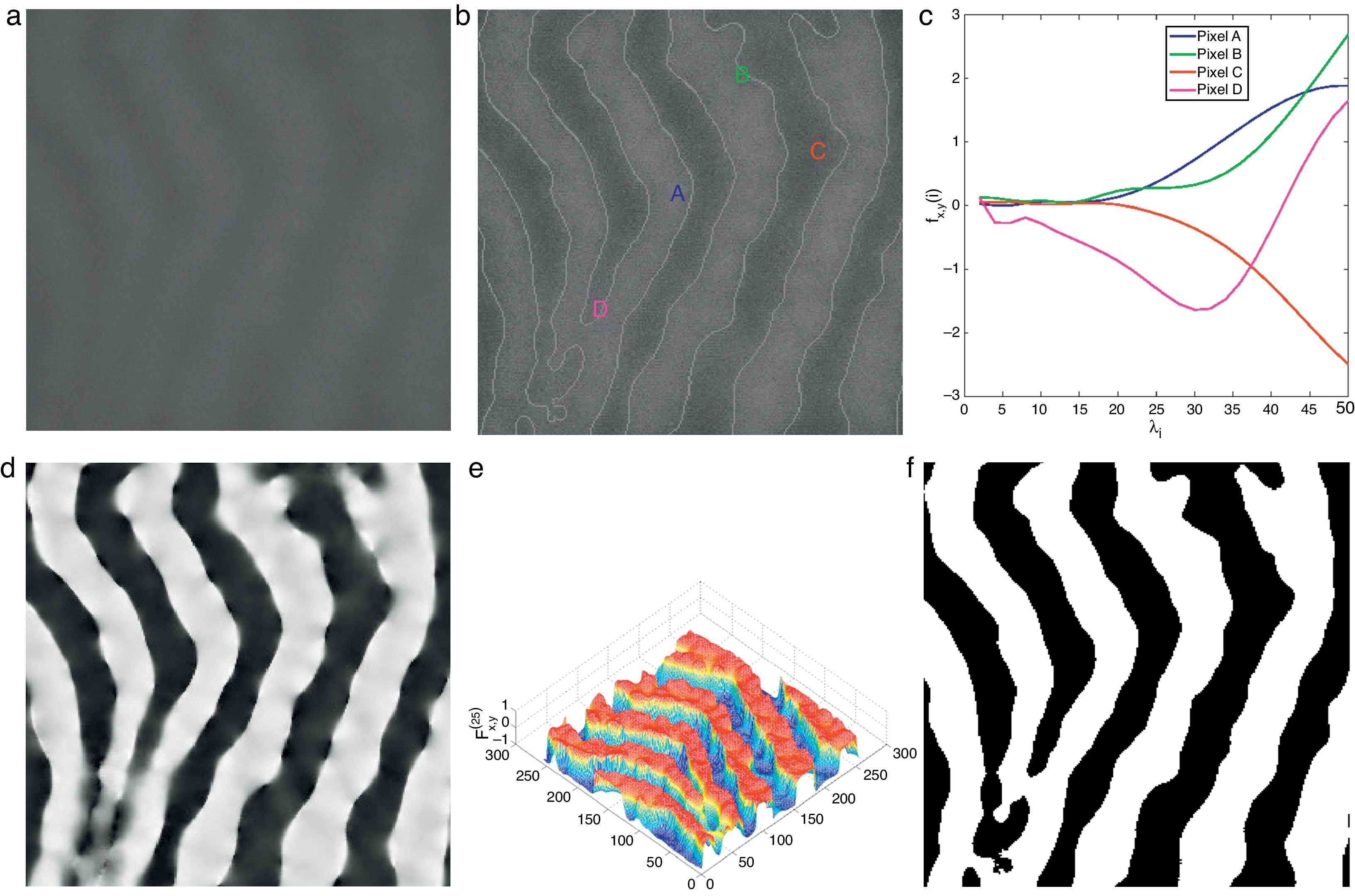
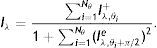
The denominator in Eq. (14) is used to compensate the fluctuations due to illumination differences over different parts of the image. In Fig. 4, Gabor filter responses according to Eq. (14) are shown for λi=2i, i=1, 2, …, Nλ=25. From the feature vectors shown in Fig. 4(c), the entries of feature vectors are mostly positive on gland regions, and negative in inter-gland regions. The average feature F(Nλ) is computed as
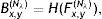
which is demonstrated in Fig. 4(d) and (e) where the discrimination between gland and inter-gland regions are clear. Using Eq. (15), the final binary image B(Nλ) is computed according towhere H(·) is defined in Eq. (12). The result of binarization according Eq. (16) is shown in Fig. 4(f) and boundaries are overlayed onto input image in Fig. 4(b). It is clear that merging information from different values of λ improves the discrimination between gland and inter-gland regions.
 over different spatial locations for Nλ=25 and Nθ=72: (a) input 256×256 pixels IR image cropped from Fig. 1(a); (b) contrast enhanced IR image on which the boundary pixels detected from binary image in (f) is overlayed and corresponding pixel locations over which Gabor filter responses are observed; (c) Gabor filter responses of pixels shown in (b) according to Eq. (14); (d) Gabor filter response of (a) computed according to Eq. (15); (e) surface plot of (d); (f) binarized Gabor filter response B(Nλ) according to Eq. (16). (For interpretation of color in the artwork, the reader is referred to the web version of the article.)")
Demonstration of Gabor filter responses according to Eq. (14) over different spatial locations for Nλ=25 and Nθ=72: (a) input 256×256 pixels IR image cropped from Fig. 1(a); (b) contrast enhanced IR image on which the boundary pixels detected from binary image in (f) is overlayed and corresponding pixel locations over which Gabor filter responses are observed; (c) Gabor filter responses of pixels shown in (b) according to Eq. (14); (d) Gabor filter response of (a) computed according to Eq. (15); (e) surface plot of (d); (f) binarized Gabor filter response B(Nλ) according to Eq. (16). (For interpretation of color in the artwork, the reader is referred to the web version of the article.)
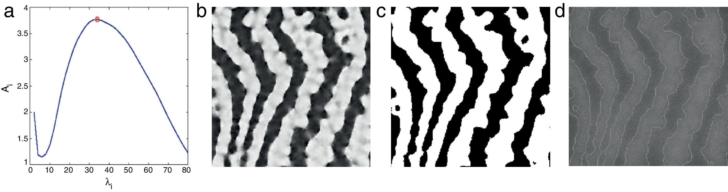
The performance of the binarization in Eq. (16) mainly depends on the discrete set of λ. The binarization results obtained by exploiting different sets of λ show various trade-offs yielded between spatial-detail preservation and noise reduction. One can specify a range for λ according to required trade-off between spatial-detail preservation and noise reduction. However, in order to achieve a fully automated system which automatically selects the maximum value of λ, λmax from a discrete set of {λi}, the first local maxima of the following measure is considered
where Si,1={(x,y),Bx,y(i)=1} and Si,0={(x,y),Bx,y(i)=0} are sets of pixels referring to regions with binary values of 1 (gland) and 0 (inter-gland), respectively, and |Si,1| is the cardinality of set Si,1. The above equation simply subtracts average responses over estimated gland and inter-gland regions which is expected to have high values for a good global partitioning of gland and inter-gland regions. In Fig. 5, automatic selection of λmax according to Eq. (17) from a set of {λi=2i, i=1, …, Nλ=40} is demonstrated. λmax=34 is dynamically selected and the resultant binary image is shown in Fig. 5(c).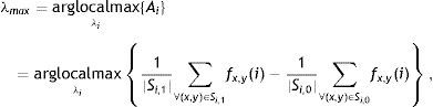
 from a discritized set λi=2i, i=1, 2, …, Nλ=40: (a) plot of energy function Ai computed according to Eq. (17) and selecting the local maxima which is labelled with red circle; (b) average Gabor feature response according to Eq. (15); (c) binarization result according to Eq. (16); (d) corresponding 256×256 pixels input image with superimposed boundaries detected from binary image in (c). (For interpretation of color in the artwork, the reader is referred to the web version of the article.)")
Selecting λmax according to Eq. (17) from a discritized set λi=2i, i=1, 2, …, Nλ=40: (a) plot of energy function Ai computed according to Eq. (17) and selecting the local maxima which is labelled with red circle; (b) average Gabor feature response according to Eq. (15); (c) binarization result according to Eq. (16); (d) corresponding 256×256 pixels input image with superimposed boundaries detected from binary image in (c). (For interpretation of color in the artwork, the reader is referred to the web version of the article.)
Since the λ is spatial wavelength, the average gland width of the input image can be estimaed as λmax/2 which.
Finding Mid-lines Using Binary SkeletonizationThe proposed method produces a binary image where gland and inter-gland regions are represented by binary 1s and 0s, respectively. The lengths and widths of gland and inter-gland structures are estimated using mid-lines of structures. The mid-lines also make it easy to assess the gland and inter-gland structure.
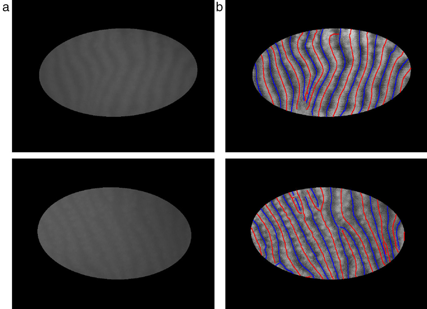
The mid-lines of gland and inter-gland regions are obtained using binary skeletonization.16 The aim of the skeletonization is to extract a region-based shape feature representing the general form of forground object.16 Skeletonization is applied on gland and inter-gland regions to obtain the corresponding mid-lines. It is worth to note that further pruning can be applied on final result of skeletonization, however, this will come with extra computational cost. In pruning, the fast marching method widely used in level set applications is augmented by computing the paramterized boundary location every pixel came from during the boundary evolution.17 The resulting parameter field is then thresholded to produce the skeleton branches created by boundary features of a given size. The threshold for each image is selected as λmax computed as according to Eq. (17). In Fig. 6, automatically detected mid-lines of gland and inter-gland regions on input images in (a) are shown with red and blue lines, respectively, in (b).
 corresponding input 576×768 pixels image with superimposed region of interest and (b) detected mid-lines of gland and inter-gland regions labeled with red and blue lines, respectively, using skeletonization. (For interpretation of color in the artwork, the reader is referred to the web version of the article.)")
Finding mid-lines of gland and inter-gland regions: (a) corresponding input 576×768 pixels image with superimposed region of interest and (b) detected mid-lines of gland and inter-gland regions labeled with red and blue lines, respectively, using skeletonization. (For interpretation of color in the artwork, the reader is referred to the web version of the article.)
The detected mid-lines of gland and inter-gland regions are used to extract features which are further combined together with support vector machines classifier to seperate “healthy”, “intermediate” and “unhealthy” images. For each detected mid-line pixel of gland and inter-gland regions located at spatial location (xp, yp), principal orientation θp and width λp/2 are recorded. Entropy of spatial distribution (x–y distribution) and entropy of orientation versus width distribution of mid-lines of gland and inter-gland regions are used as features.
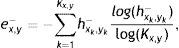
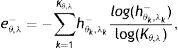
FeaturesLet hx,y+ and hx,y− be 2-D normalised spatial histograms of pixels on detected mid-lines of gland and inter-gland regions, respectively. Similarly, let hθ,λ+ and hθ,λ− be 2-D normalised histograms of principal orientation versus width of pixels on detected mid-lines of gland and inter-gland regions, respectively. Using these histograms, the following features are extracted to describe spatial distribution of gland and inter-gland mid-lines on region of interest,
where Kx,y is the number of bins, (xk, yk) is kth bin center, and ex,y+ and ex,y− are, respectively, normalized entropies representing spatial features of gland and inter-gland mid-lines. In this study, x and y axis of region of interest are uniformly quantized into 10 levels, i.e., K=10×10=100. Similarly, in order to describe the principal orientation and width of gland and inter-gland mid-lines, the following features are usedwhere Kθ,λ=Nθ×Nλ is the number of bins, (θk, λk) is kth bin center, and eθ,λ+ and eθ,λ− are, respectively, normalized entropies of principal orientation and width features of gland and inter-gland mid-lines.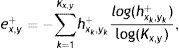

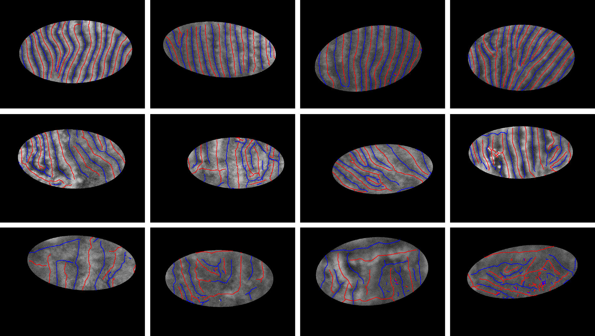
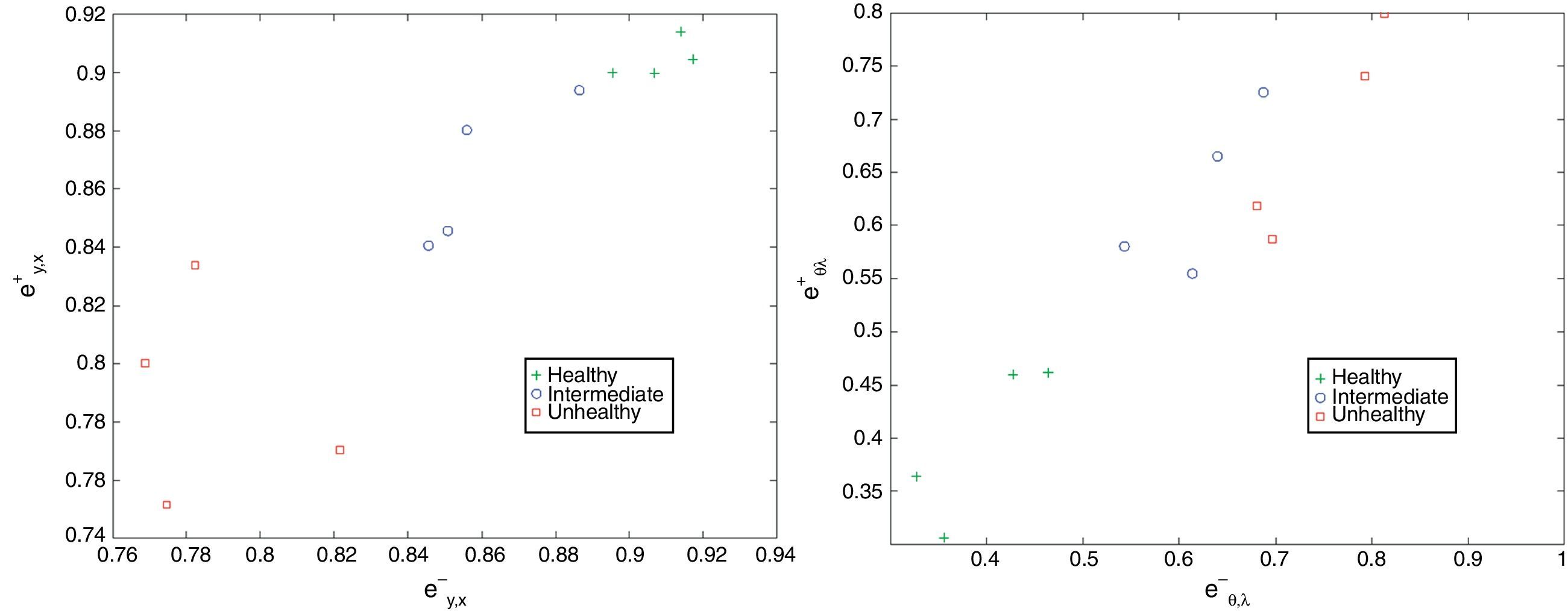
In Fig. 7, detected mid-lines are shown for samples from “healthy” (the first row), “intermediate” (the second row), and “unhealthy” (the third row) images. The corresponding scatter plots of features are shown in Fig. 8. It is clear that, the features can be used to separate the images into classes. The features measure how uniformly the gland and inter-gland mid-line pixels are distributed. For instance, for an healthy eye, the gland and inter-gland mid-lines should be uniformly distributed over the region of interest. This wil result in high entropy values. Meanwhile, they should be elongated in a certain direction and with almost homogenous widths. This observation should result in low entropy values. The scatter plots reflect these observations.
, “intermediate” (the second row), and “unhealthy” (the third row) images. (For interpretation of color in the artwork, the reader is referred to the web version of the article.)")
 ex,y− versus ex,y+; and (b) eθ,λ− versus eθ,λ+.")
Scatter plots of detected features from “healthy”, “intermediate”, and “unhealthy” images shown in Fig. 7: (a) ex,y− versus ex,y+; and (b) eθ,λ− versus eθ,λ+.
For a given image, the features ex,y+, ex,y−, eθ,λ+ and eθ,λ− are extracted. These features are used to train a 3-class SVM from training samples of “healthy”, “intermediate”, and “unhealthy” images. In the implementation of three-class SVM, regular two-class SVM is used with one-versus-all strategy.18
Results and DiscussionsSubjects, Equipment, and GradingA set of 131 IR images of resolution 576×768 (height×width) pixels graded as healthy (26 images), intermediate (76 images), and unhealthy (29 images) by an expert is used in experiments. The images collected from the dry eye clinic and the general eye clinic of Singapore National Eye Center. Written informed consents were obtained. The study was approved by the Singhealth Centralised Institutional Review Board and adhered to the tenets of the Declaration of Helsinki.
The patient's chin was positioned on the chin rest with the forehead against head rest of a slit-lamp biomicroscope Topcon SL-7 (Topcon Corporation, Tokyo, Japan). This was equipped with an infrared transmitting filter and an infrared video camera (XC-ST5CE0, Sony, Tokyo, Japan). The upper eyelid of the patient was everted to expose the inner conjunctiva and the embedded meibomian glands. This is a standard procedure and causes no pain to the patient. Images were acquired using a 10x slit-lamp magnification. Care was taken to obtain the best focus as well as to avoid reflections on the inner eyelid surface. The lower eyelid was not imaged in this report because in the authors’ experience, it was easier to uniformly focus the image of the tarsal plate in the upper eyelid.
The mid-lines of gland and inter-gland regions are represented as set of connected straight lines. The mid-lines are labeled by an expert. Furthermore, for each image a region of interest containing glandular tissue which is roughly represented as a ellipse shape is identified by the expert.
Implementation Details and Performance MeasuresIn experiments, automatic gland and inter-gland region identification performance of the proposed algorithm is tested. The settings of Nθ=36 and {λi=5i, i=1, …, 24} are used.
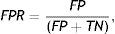
The proposed method detects the gland and inter-gland regions as well as their mid-lines using binary skeletonization. The detected mid-lines are compared with ground-truth mid-lines. In comparisons, the detection performance for an input image is computed using true positive rate (TPR) or sensitivity and false positive positive rate (FPR). The measurements are defined as
where true positive (TP) is the number of gland mid-line pixels which are correctly detected, true negative (TN) is the number of inter-gland mid-line pixels which are correctly detected, false positive (FP) is the number of inter-gland mid-line or non-gland pixels which are detected as gland mid-line pixel, and false negative (FN) is the number of gland mid-line or non-gland pixels which are detected as inter-gland mid-line. A pixel which is detected either gland mid-line or inter-gland mid-line is assigned to the label of ground-truth pixel if the ground truth pixel is found within a spatial radius r of detected pixel. This is required mainly due to compensate for labeling errors as it is quite difficult to choose mid-lines of regions even for an expert. In experiments r=λmax/2 pixels are used.Quantitative Analysis on Mid-line Detection Performance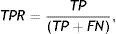
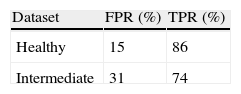
The average detection performance results on healthy and intermediate images are reported in Table 1. The unhealthy images are not considered as they don’t have regular gland and inter-gland structure. The results indicate that the algorithm can achieve 86% and 74% true positive rates on healthy and intermediate datasets, respectively. Meanwhile, the false positive rates are 15% and 31% on healthy and intermediate datasets, respectively. The ground-truth labelings from expert also have some errors. This further decreases the quantified performance.
When the correct detection rate, which is the ratio of correctly detected mid-line pixels and the total number of mid-line pixels for each category, is considered the proposed algorithm can achieve correct detection rates of 94% and 98% on gland and inter-gland mid-lines, respectively, of healthy images dataset. Meanwhile on intermediate images dataset, the proposed algorithm can achieve 92% and 97% detection rates on gland and inter-gland mid-lines, respectively. False detections are generally due to imperfect skeletonization, image artefacts and errors in ground-truth labelings.
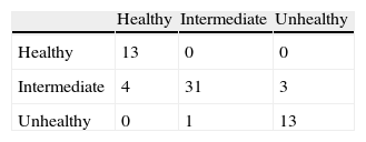
Quantitative Analysis on Image Classification PerformanceThe half of images in each class are used for training three-class SVM with the strategy of one-vs-all. Gaussian radial basis function with scaling factor of 1.5 is used as a kernel function of SVM. The other half of images in each class are used for validating three-class SVM. In each experiment, the samples from classes are randomly selected. The experiment is repeated 1000 times and the results are shown in Table 2 as a confusion matrix.
The results show that the proposed method can achieve 88% accuracy in correctly classifying images into “healthy”, “intermediate” and “unhealthy” classes. Although most of the times intermediate images are correctly classified, 7 images out of 38 intermediate images are incorrectly classified. This is mainly due to the reason that intermediate images fall in between categories of “healthy” and “unhealthy” images and distinction between extracted features of these classes may not always be clear. It is worth to note that the classification performance raises up to 100% accuracy for classifying images into “healthy” and “unhealthy” classes. The results show that extracted features from detected mid-lines of gland and inter-gland regions are adequate to asses the images.
DiscussionsThe method is completely automated and requires no parameter tuning from the user except sampling resolution of continuous parameters used in Gabor filtering. The default sampling of continuous parameters produces satisfactory results. We have tested higher resolution sampling of the parameters, however, no noticable difference is observed in terms of gland and inter-gland region detection and classification performances. Sampling resolution of continuous parameters can be set once according to the image resolution.
The proposed algorithm can only perform two-class segmentation, i.e., a pixel of input IR image is segmented as either belonging to gland or inter-gland regions. Pixels out of glandular tissue are also automatically classified into one of the two classes which produces false detections. Thus, it is necessary to achieve three-class segmentation representing gland, inter-gland and non-gland regions. As a future work, supervised learning methods will be investigated to achieve three-class segmentation. The results of three class segmentation can be merged with gland and inter-gland mid-line detection algorithm proposed in this paper. This will improve the correct detection rate which will result in performance improvement in terms of correct classification into “healthy”, “intermediate” and “unhealthy” classes.
High-level features such as gland and inter-gland widths and lengths can be used in assessing Meibomian gland dysfunction. Since the settings such as magnification factor in IR imaging can be changed between different patients, the extracted features should be normalized according to glandular tissue in consideration. Thus, it is important to automatically identify glandular tissue region from input images. For this purpose, supervised learning methods can be used to automatically identify glandular tissue region from input images.
The proposed algorithm detects reflections in IR images as glandular structures provided that the corresponding reflections cover image regions which have surface area larger than the square of minimum spatial wavelength used in Gabor filtering process. However, this will have minor effect on the image classification if the the reflections cover small regions. As a future work, we plan to improve the algorithm to automatically identify the reflection regiongs to exclude corresponding pixels from further anlaysis.
The algorithm is designed for analysis of upper eyelid images. As a future work, the performance of the algorithm will be tested on lower eyelid images.
ConclusionWe have introduced a method for automated gland and inter-gland regions identification from IR images of Meibography. The identified regions are used to detect the mid-lines of gland and inter-gland regions. The algorithm can correctly detect 94% and 98% of mid-line pixels of gland and inter-gland regions, respectively, on healthy images. On intermediate images, correct detection rates of 92% and 97% of mid-line pixels of gland and inter-gland regions, respectively, are achieved.
Extracted features from detected mid-line pixels are used to perform automated image classification. Accuracy of 88% is achieved in classying images into one of “healthy”, “intermediate” and “unhealthy” classes. Meanwhile, the algorithm can achieve 100% accuracy in seperating “healthy” and “unhealthy” images.
Conflicts of interestThe authors have no conflicts of interest to declare.
This work is supported in part by the Agency for Science, Technology, and Research (A*STAR) of Singapore, Biomedical Research Council/Translational Clinical Research Programme 2010 grant 10/1/06/19/670, and National Medical Research Council individual grants NMRC/1206/2009, NMRC/CSA/013/2009, and NMRC/CG/SERI/2010.


