

We review the psychophysics of the spatio-temporal contrast sensitivity in the cardinal directions of the colour space and their correlation with those neural characteristics of the visual system that limit the ability to perform contrast detection or pattern-resolution tasks. We focus our attention particularly on the influence of luminance level, spatial extent and spatial location of the stimuli - factors that determine the characteristics of the physiological mechanisms underlying detection. Optical factors do obviously play a role, but we will refer to them only briefly. Contrast sensitivity measurements are often used in clinical practice as a method to detect, at their early stages, a variety of pathologies affecting the visual system, but their usefulness is very limited due to several reasons. We suggest some considerations about stimuli characteristics that should be taken into account in order to improve the performance of this kind of measurement.
Se revisa la psicofísica sobre la sensibilidad al contraste con patrones espacio-temporales en las direcciones cardinales del espacio de color y su relación con las características neuronales del sistema visual que limitan la habilidad para realizar una tarea de detección de contraste o de resolución de patrones. La atención se centra especialmente en la influencia del nivel de luminancia, el tamaño y la localización espacial de los estímulos, en la medida que estos son los factores más importantes que determinan las características de los mecanismos fisiológicos que median la detección. Obviamente, los factores ópticos también juegan un papel en el conjunto del sistema visual, pero nos referiremos a ellos sólo brevemente. Las medidas de sensibilidad al contraste son a menudo usadas en clínica como método para detectar, en un estado temprano, una amplia variedad de patologías del sistema visual, pero su utilidad en la práctica es bastante limitada por diferentes razones. Sugerimos que ciertas consideraciones sobre los estímulos deberían ser tenidas en cuenta si se quiere mejorar las prestaciones actuales de este tipo de medidas.
During the last three decades, the possibility of early detection of a variety of pathologies affecting the visual system by means of the measurement of spatial and temporal contrast sensitivity functions —CSFs- has been thoroughly explored.1-16 (Burr D, et al. IOVS 2003;44: ARVO E-Abstract 3193). It has been shown, however, that the usefulness of these functions is rather limited in practice, for several reasons. In the first place, measurements are often limited to the fovea, whilst anatomical damage and functional loss frequently begin outside this region [see, for example, F. Rowe's book17]. In fact, different perimetry techniques have been developed to asses the sensitivity of the visual system at different points of the visual field, but instruments performing contrast sensitivity tests with sinusoidal gratings are scarce and, in fact, none of them explores a sufficiently large frequency range, neither in the spatial nor in the temporal domain.5,16,18-20 However, exploring the frequency range could be useful, since damage caused by different pathologies may affect different regions of the frequency spectrum.1,3,21-22 (Burr D, et al. IOVS 2003;44: ARVO E-Abstract 3193). In the second place, contrast sensitivity measurements are almost exclusively confined to those made with achromatic gratings, although it has been shown that many pathologies cause colour- discrimination losses.9,23-29 Even those instruments that are capable of measuring the chromatic contrast sensitivity functions (cCSFs) at the fovea are not in current use. It is worth pointing out that the chromatic gratings used for this sort of measurements cannot be modulated along any direction in the colour space, since the aim of the experiment is to ensure that the stimulus shall be detected by a particular chromatic mechanism, be it the red-green mechanism physiologically mediated by the Parvo pathway or a blue-yellow mechanism mediated by the Konio pathway. This requirement is relevant because, according to the minimal-redundancy principle, the detection of early functional losses is more likely to be successful when the test employed is selective for a given mechanism (though which mechanism may be unimportant) than when it is not selective.30 Of course, evidence supporting the diagnostic usefulness of the chromatic contrast sensitivity functions can be found in the literature2,6-11,14-15 (Burr D, et al. IOVS 2003;44: ARVO E-Abstract 3193) but their use in everyday clinical practice is basically negligible. In the third and last place, when contrast sensitivity measures are made, the spatio-temporal characteristics of the stimuli are usually too restrictive. Most frequently, contrast sensitivity is measured with stationary spatial gratings (that is, with zero temporal frequency, and often also with a single fixed spatial frequency) or with spatially uniform temporal gratings (that is, with zero spatial frequency and often also with a single fixed temporal frequency). However, it is well known that using specific combinations of spatial and temporal frequencies in achromatic gratings we may separate the detections made by an achromatic mechanism of magnocellular origin from those made by a Parvocellular achromatic mechanism.31-32 However, only the FDT (Frequency Doubling Technology) perimeter uses this type of spatio-temporal patterns for contrast sensitivity measurements, even if it is only a particular combination of frequencies which is tested, combination that, in fact, isolates the magnocellular pathway.33-34
In this paper, we review the essential psychophysics of the spatio-temporal contrast sensitivity functions in the cardinal directions of the colour space and some of the neural characteristics of the visual system that limit the ability to perform contrast detection or pattern resolution tasks. We will focus our attention particularly on the influence of the luminance level, which determines the adaptation state of the visual system, and the spatio-chromatic characteristics of the stimuli (including the spatial location), which determine the physiological mechanisms underlying detection. Optical factors do obviously play a role, but we will refer to these only briefly.
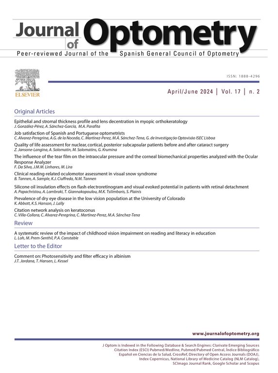
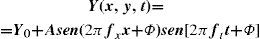
Some Preliminary ConceptsContrast is the physical parameter describing the magnitude of the luminance variations around the mean in a scene. The choice of an appropriate metric to measure contrast is not a trivial question, since in any particular scene luminance may change from point to point in complex ways. Fortunately, this is not the case with the visual stimuli used to assess the condition of a subject's visual system. Usually, the stimulus is a single object of uniform luminance presented against a uniform background (Figure 1A) or a periodical pattern, with sinusoidal (Figure 1B) or eventually square profile (Figure 1C). If the stimulus is aperiodical, contrast is simply defined as:
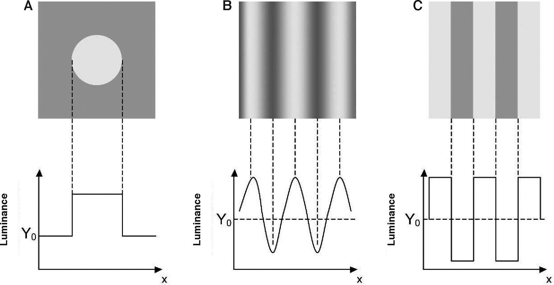
where ΔY is the luminance amplitude of the stimulus placed against the luminance Y0 (i.e., the background), provided that Y0≠0. This definition is known as Weber's contrast. If the stimulus is a spatially periodical pattern (or grating), it is defined by its spatial frequency, which is the number of cycles per unit of subtended angle. The luminance profile of a sinusoidal grating of frequency f (measured in cycles per degree, cpd) oriented along a spatial direction defined by the angle θ (Figure 2) can be written as:where Y0 is the mean luminance of the grating, A is its amplitude and fx and fy are its spatial frequencies along the x and y directions, respectively; that is:or, equivalently:


The value of the phase, Φ, determines the luminance at the origin of coordinates (x=0, y=0). If Φ is zero or a multiple or π rad, luminance is zero at the origin and the pattern has odd symmetry, whereas if Φ is π/2 rad or an odd multiple of π/2 rad, luminance is maximum at the origin and the pattern has even symmetry. Note that the grating shown in figure 1B has fy=0 and Φ=π/2 rad. Contrast is defined in this case as follows:
that is:

This expression is known as Michaelson's contrast. This definition can be applied to any periodical pattern, no matter if sinusoidal, square or any other type. Contrast sensitivity is the inverse of the minimum contrast necessary to detect an object against a background or to distinguish a spatially modulated pattern from a uniform stimulus (threshold contrast). In this paper, we will deal primarily with contrast sensitivity measured with sinusoidal patterns.
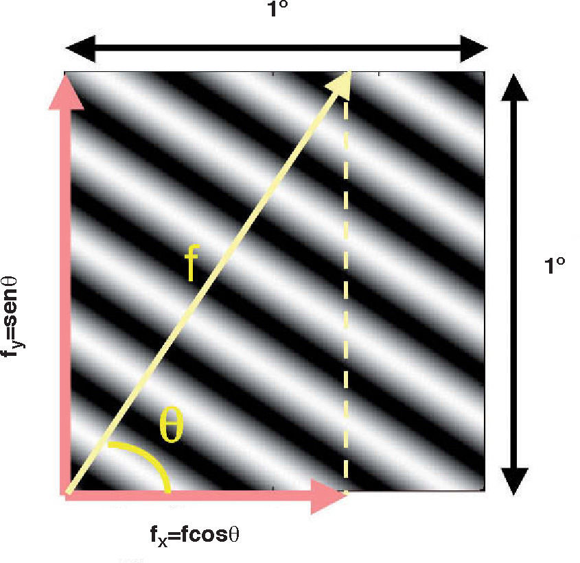
The Achromatic Contrast Sensitivity Function: CsFContrast sensitivity is a function of the spatial frequency (f) and the orientation (θ) of the stimulus; that is why we talk of the Contrast Sensitivity Function (or its abbreviation CSF). Figure 3 shows the typical shape of this curve for a subject with a normal visual system when θ=π/2 rad. At photopic levels, the curve peaks at 3-5 cpd and drops for both low and high frequencies, giving a typical band-pass shape. The cut-off frequency (or resolution), defined as the highest possible frequency that can be just detected with unit Michaelson's contrast, is about 40-60 cpd. In optics, a well-known function of spatial frequency used to characterize the quality of an imaging system is the Modulation Transfer Function (MTF for short), which can be measured by obtaining the image (output) produced by the system of a sinusoidal pattern of frequency f, orientation θ and contrast Cin(f,θ) (input), since it can be shown that the following equality holds [see, for example, J.D. Gaskill's book35, Chapter 8]:
where Cout(f,θ) is the contrast of the image, which is also a sinusoid, provided the system is linear and spatially invariant. This formula may be read as the contrast transmittance of a filter. If the visual system is treated globally as a linear, spatially invariant, imaging system and if it is assumed that, at threshold, the output contrast must be constant, i.e., independent of spatial frequency, it is easy to demonstrate that the MTF and the CSF of the visual system must be proportional. In fact, if the input is a threshold contrast grating, the MTF can be written as:We are assuming that Cthres,out(f,θ) is an unknown constant, let us say R0. Then (8) becomesBut the CSF is the inverse of the contrast threshold, and therefore


Thus, both functions have the same shape and differ only in an unknown global factor. The MTF and the CSF may be defined not only for the global visual system, but also for its constituent parts. Let us consider, in particular, that the visual system is formed by two systems acting in succession: the optical system and the neural system. Since the MTF of the global system is the product of the MTFs of its optical and neural parts, by applying Equation 10 it follows that:

Given that the MTF of any optical system is low-pass shaped, the band-pass form of the CSF of the visual system must be due to the neural processing of the image formed on the mosaic of photoreceptors. As a matter of fact, the first experimental measurement of the optical MTF in vivo was achieved by using Equation 11, where the neural CSF was measured with gratings formed directly on the retina by means of interferometric methods, which bypass the optical system.36-37 Modern measurements of the optical MTF are based on an objective procedure, does not relay on contrast-threshold measurements. As can be seen in figure 4, however, the results obtained with this technique do not differ in anything essential from those derived with an interferometric method.38
 and by an objective method (double-pass method: red curve). The blue line shows the diffraction-limited MTF.")
Empirical MTF measured with a 3mm pupil by a subjective method (interferometric method: green curve) and by an objective method (double-pass method: red curve). The blue line shows the diffraction-limited MTF.
At any frequency, contrast sensitivity is basically the same at θ=0 rad and θ=π/2 rad, but a significant sensitivity reduction is found at around θ=π/4 rad, especially for higher frequencies, which results in a loss of resolution when measurements are carried out with gratings having this orientation.39-41 This behaviour of the visual system is well known, and has been named the “oblique effect”. Although the exact causes of this effect have been elusive for a long time, at present it seems clear that it is cortical in origin.42 In what follows, we will assume that there are no reasons of optical nature that make it necessary to introduce an explicit dependence of the MTF on orientation—a fact which would also ultimately affect the CSF—and we will discuss only the effect of frequency on the CSF, keeping stimulus orientation fi0xed at a value of θ=π/2 rad.
Factors Determining Contrast SensitivityContrast sensitivity depends upon many factors having both optical and neural origin. Included among the most relevant optical factors, due to the fact that they determine the optical MTF, are pupil diameter,36,43 eccentricity44,45 and, naturally, the refractive state of the subject.36,46 There is abundant literature about these questions that the interested reader may refer to [see, for example, the chapter by L. Thibos in K. De Valois’ book47].
Among the neural factors, which are those that give more information about the nature of the physiological mechanisms mediating the detection of achromatic patterns, we will consider particularly three: mean luminance, stimulus size and eccentricity. Mean luminance determines the adaptation state of the visual system, size determines the number of cycles that the stimulus comprises, and eccentricity determines the characteristics of the mosaics of sensors acting in cascade to perform a given visual task.
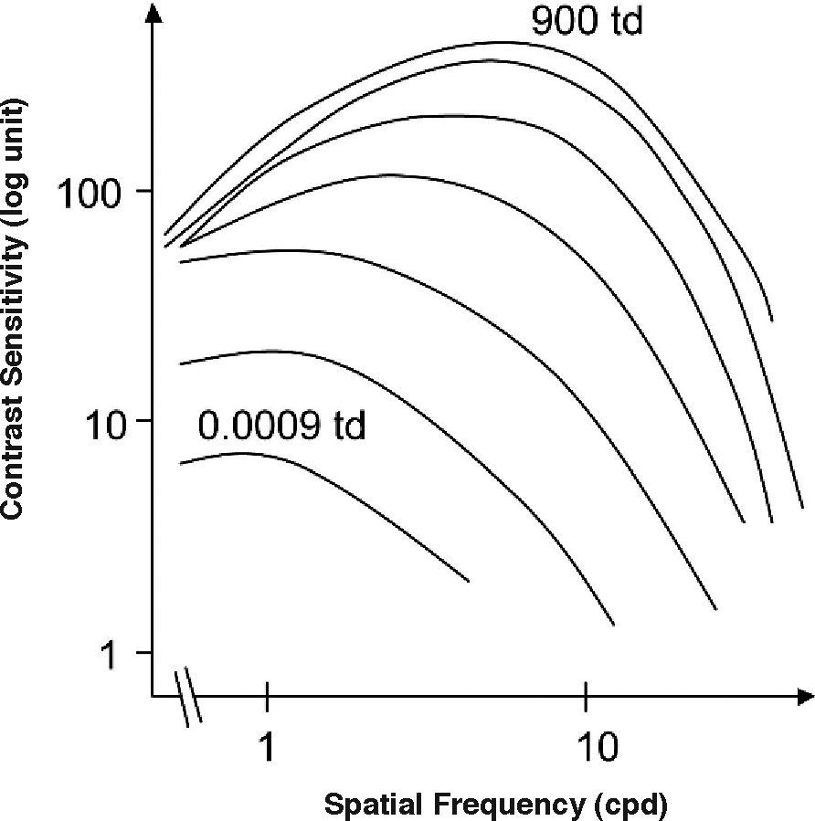
LuminanceFigure 5 shows several CSFs measured at different mean luminance levels. When the mean luminance is high, the shape of the CSF is that of a band-pass filter, as we already know. As mean luminance is progressively reduced to scoto-pic level, both sensitivity and resolution decrease and the shape of the CSF progressively becomes that of a low-pass filter. For even lower mean luminance values, sensitivity and resolution still decrease, until the CSF becomes fully low-pass shaped. Above a certain mean luminance value, adaptation at the low-frequency range is governed by Weber's law. It can be seen, in fact, that when frequency approaches zero, sensitivity and, therefore, threshold contrast don’t depend on the mean luminance. Or, in other words, the amplitude threshold is proportional to the mean luminance. In the high-frequency region, however, contrast thresholds decrease with the square root of the mean luminance, because the amplitude threshold increases with the square root of the mean luminance, a behaviour that is known as the De Vries-Rose law. The frontier luminance between the De Vries-Rose and Weber laws increases with the square of frequency, according to the constant-flux hypothesis.48-50 A classical related effect is the well-known dependences of visual acuity with luminance for high-contrast targets and with contrast for high (photopic) luminance levels [see, for example, the chapter by H. D. Bedell in Norton et al.’s book51].
 to a high level (top: 900 Td).")
Spatial CSFs measured at different mean luminance levels, at logarithmic steps from a low (bottom: 0.0009 Troland (Td) to a high level (top: 900 Td).
The standard photopic CSF is mediated by cells in the parvocellular pathway. This has proven to be true because the CSF of a macaque monkey that has undergone selective destruction of LGN Magno cells is not significantly different from the CSF measured before the lesion,31-32 while if the damaged cells belong to the parvocellular pathway, the contrast sensitivity decreases for all frequencies and the CSF changes from bandpass to low-pass shaped (see Figure 6, left). This result seems in apparent contradiction with the high sensitivity found for individual M cells, surpassing even that of most P cells, provided that the spatial frequency is not above 2-3 cpd (Figure 7)52. Therefore we must be careful not to identify mistakenly the global properties of a mechanism with those of its individual components, since the properties of the mechanism depend as well on how the responses of the individual components are combined to arrive to the global response.
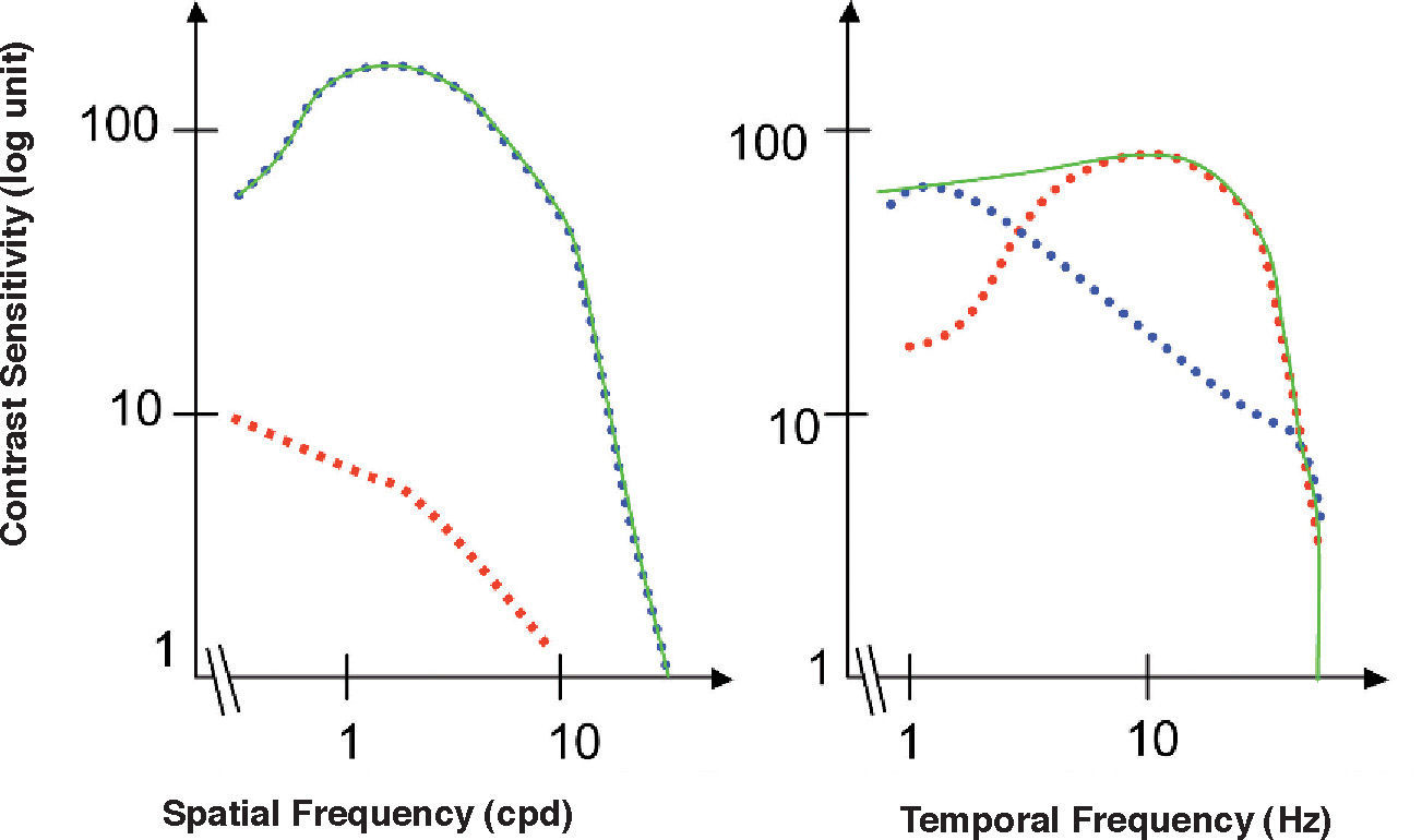
 and temporal (right) photopic CSF measured in a macaque monkey (continuous green line). The red dottedline shows magnocellular-only sensitivity, while the blue dotted-line shows parvocellular-only sensitivity.")
Standard spatial (left) and temporal (right) photopic CSF measured in a macaque monkey (continuous green line). The red dottedline shows magnocellular-only sensitivity, while the blue dotted-line shows parvocellular-only sensitivity.
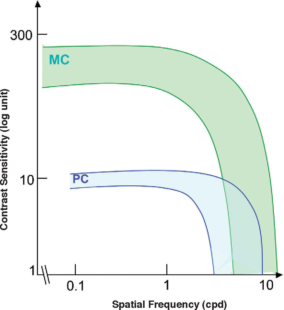
 and parvocellular (PC) cells of the macaque monkey.")
Variability of the spatial contrast sensitivity for magnocellular (MC) and parvocellular (PC) cells of the macaque monkey.
If mean luminance is reduced to the neighbourhood of the scotopic level, detection turns out to be mediated by cells of the magnocellular pathway, whose global CSF is low pass. Again, we find here contradictions with the properties of individual cells, since the individual cells’ CSFs are band-pass. However, for a dark-adapted visual system the peripheries of the receptive fields of M cells are silenced53 and the CSFs become low-pass, as for any mechanism without spatial selectivity.
Spatial Extent for Optimal StimuliIncreasing stimulus size means that more cycles of the stimulus are present. To understand what happens when the number of cycles is increased, let us remember that the cells in the striate cortex (V1) are, in the frequency domain, a set of band-pass frequency-tuned sensors, peaking at frequencies with 1-octave spacing (that is, uniformly spaced in a base-2 logarithmic scale) and constant bandwidths in octaves; that is, bandwidths proportional to the peak frequency.54-55 The global CSF of the visual system is the envelope of the responses of these sensors [see, for example, the chapter by H. R. Wilson and E Wilkinson in L. M. Chalupa and J. S. Werner's book56]. On the other hand, receptive field size and bandwidth in the frequency domain are inversely proportional, and taking into account the relationship between bandwidth and peak frequency, the same law holds for field size and peak frequency. Therefore, the receptive fields of the cortical sensors have sizes equivalent to a certain unique number of cycles. Let us assume that we are measuring a CSF with stimuli whose spatial frequencies match those the cortical sensors are tuned to; for instance, 0.5, 1, 2, 4, 8 and 16 cpd. Maximal response in the sensor tuned to a given frequency is reached only if the stimulus size matches the receptive field size. Therefore, all stimuli ought to contain certain unique number of cycles, but how many? The answer to this question depends on the sensor's bandwidth—usually assumed to be equal to 1 octave, equivalent to around 1.5 cycles—but the relevant point of this discussion is that increasing the number of cycles above this value will not increase the response of the particular sensor mediating detection of that stimulus and, therefore, it will not raise contrast sensitivity.
Note that all we have reasoned above rests on the assumption of constant sensor's bandwidth (in octaves), but the reality is that the bandwidth of cortical cells decreases from 2.5 octaves for the lowest frequencies to 1 for the highest.54-55 This is at least one of the reasons behind the increment in contrast sensitivity that is indeed found when a low-frequency stimulus increases in size to contain up to 3-4 cycles, whereas 1.5-2 cycles sets the limit for a noticeable sensitivity enhancement at high frequencies. Thus, with a stimulus subtending 5° in size, containing 2.5 cycles for a frequency of 0.5 cpd, the sensitivity would be reasonably optimized for all the frequency spectrum.
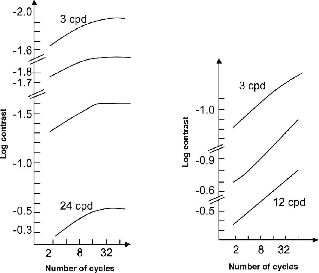
However, is this the only reason for the increase in contrast sensitivity with the number of cycles? The answer is no, since contrast sensitivity basically depends on how sensors tuned to the same stimulus add their responses. With an increasing number of cycles, more cells are stimulated and may, therefore, contribute to the detection task. The result, as shown in figure 8, is a linear increase of the contrast sensitivity (log scale) with the number of cycles, up to a maximum value that depends on spatial frequency and on whether or not the stimulus is enlarged within a spatial region with uniform sensitivity—in this case, increments in sensitivity occur at least up to 32-64 cycles—or towards regions of progressively decreasing sensitivity—the limit is then only 8-16 cycles. A reasonably uniform sensitivity is attained if the stimulus is placed at a distance proportional to the size of a cycle above the fovea. On the contrary, sensitivity decreases progressively for displacements from the fovea along the horizontal or the vertical meridian.57 These reductions in sensitivity with increasing eccentricity do not follow the same pattern neither along the two meridians, nor even along the same meridian. Given the available anatomical and physiological data for anisotropies in early visual pathways, it is quite surprising the scarcity of literature showing the functional implications that these anisotropies would have in low-level psychophysical tasks, such as simple grating detection (see, for example, the recent paper by Silva and co-workers58). The distance between stimulus location and fovea is an extraordinarily relevant factor to which we will shortly pay the necessary attention.

Contrast sensitivity as a function of the number of cycles contained in the grating patch, for different spatial frequencies. The figure on the left-hand side shows the results for grating patches located within a thin vertical strip centered on the fixation point, and the figure on the right-hand side shows the results for grating patches located within a horizontal strip whose center was 42 periods vertically above the fixation point. All grating patches were centered in the strip within which they would appear. The orientation of the bars in each grating patch was perpendicular to the orientation of the strip.
A related, though minor, problem is that stimulus size distorts the frequency spectrum of the stimulus. A sinusoidal stimulus of infinite size is described by a single frequency, but if the stimulus is shown within a window that limits it in size, the frequency spectrum “spreads” around the nominal frequency of the grating. This spread may increase the probability of obtaining responses from sensors tuned to frequencies different from the nominal frequency of the grating, causing a consistent increase in contrast sensitivity. Given that the frequency spread increases with decreasing window size, increments of the stimulus size would, in this aspect, decrease the summation between neighbouring sensors in the frequency domain, counteracting the effects due to a closest match with the receptive field of a single sensor and to the summation between spatially neighbouring sensors tuned to the same frequency range [for a more detailed discussion on this point see Graham's book,59 chapter 5].
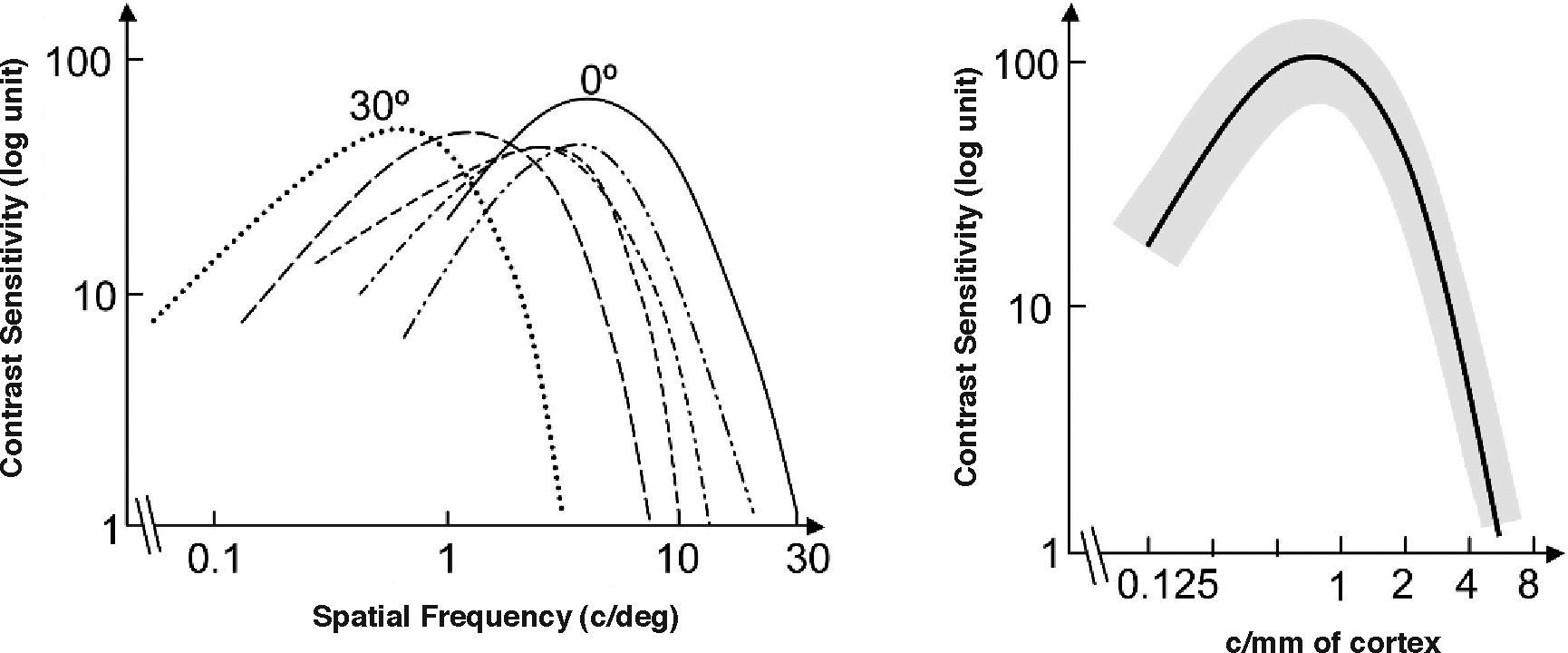
Spatial Location (eccentricity)If we use the same set of stimuli (same frequencies and sizes) to measure a CSF at fovea and at a given eccentricity E, we observe that the CSF shifts towards lower frequencies and sensitivities with increasing E, as illustrated in figure 9.60*Let us assume now that the stimuli are spatially scaled by a factor M, which depends on the eccentricity. Scaling an image by a factor M means increasing its size by a factor M, so that the number of cycles remains unchanged and the spatial frequency decreases by a factor 1/M. Under these conditions, we would obtain at eccentricity E a CSF with the same shape as that obtained at the fovea but shifted towards the lower frequencies (see Figure 10, left), without any change in overall sensitivity.60-61 This eccentricity-adapted scaling factor M is the cortical magnification at that eccentricity. Cortical magnification is the size of the cortex area activated by a stimulus subtending 1° in the visual field. Although different formulae are possible, the change of cortical magnification with eccentricity is reasonably well fitted by the following equation:62-63
where MF is the cortical magnification at fovea, and E2 is the eccentricity value for which the cortical magnification equals half of the value observed at fovea. Performance in certain spatial tasks deteriorates with eccentricity in accordance with cortical magnification, which would mean that that particular task is not limited by the sampling at the retina, but by that of the cortex. Tasks exhibiting this behaviour yield extraordinarily high resolution values—of around a few seconds of arc—justifying their global name of “hyperacuities”. Well known hyperacuity tasks are the Vernier acuity or the bisection acuity [see for example the chapter by M. J. Morgan in D. Regan's book64].
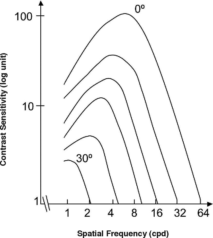
.")
Dependence of the spatial CSF with eccentricity (top: 0°, bottom: 30°).
 when the stimuli are scaled by the eccentricity-dependent cortical magnification factor M. In the figure on the left-hand side, frequency is measured in cpd and in that on the right-hand side, it is given in cycles/millimetre of cortex (see text for details).")
Dependence of the spatial CSF with eccentricity, (left: 30°; right: 0°) when the stimuli are scaled by the eccentricity-dependent cortical magnification factor M. In the figure on the left-hand side, frequency is measured in cpd and in that on the right-hand side, it is given in cycles/millimetre of cortex (see text for details).
The consequence of scaling the stimulus is that the retinotopic projection of a stimulus of size s and frequency f centered at the fovea, and that of a stimulus of size s-M(E) and frequency f/M(E) centered at eccentricity E, have the same size on the striate cortex, and the same spatial frequency if measured in cycles/millimetres of cortex (instead of in cycles/degree of visual angle). If we use this frequency unit, we would expect CSFs measured at these two spatial locations to collapse to the same curve, and this is indeed what happens, as shown in figure 10, right.60 This is an extraordinarily important result, because it shows that the visual cortex is a “homogeneous” system, although paradoxically, the visual system as a whole is not a spatially invariant one.
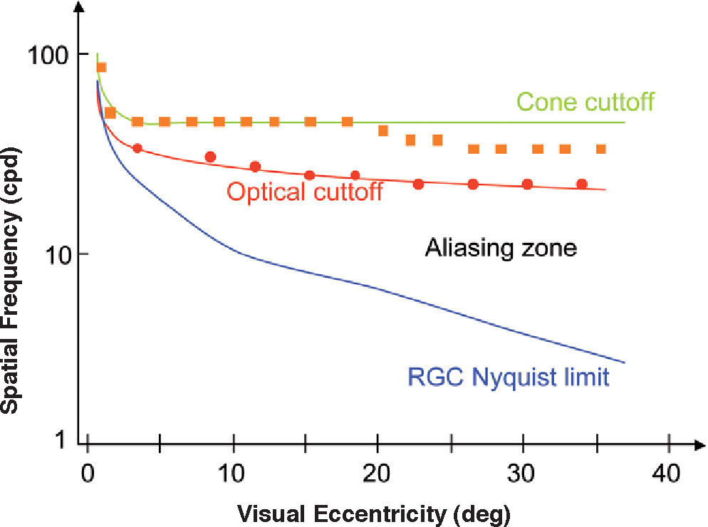
The shift of the CSF towards the low frequencies is consistent with the well-known reduction in visual acuity that is observed with increasing eccentricity [you may refer again to Bedell's chapter in Norton et al.’s book51]. Visual acuity, understood as the ability to resolve a pattern, is limited by the Nyquist frequency; i.e., that of the mosaic formed by Parvo ganglion cells. At the fovea, since the aperture of a single cone measures is 0.5min of arc and each ganglion cell receives inputs from a single cone, this results in a sampling frequency of 120 cpd and, therefore, in a Nyquist frequency of 60 cpd. The visual acuity of normal subjects is, on average, slightly lower (let us say about 1.5) provided it has been measured with a square grating of unit contrast (Foucault grating); this means that half a cycle of the grating—the smallest detail—would subtend 0.7min and hence a cycle would subtend 1.4 min, resulting in a frequency of 40 cpd. The Foveal Nyquist frequency is of the same order of magnitude as the detection limit set by the eye's optics—that is, the cut-off frequency of the MTF. Outside the fovea, as we move towards the periphery, the Nyquist frequency at ganglion-cell level decreases faster than the cut-off frequency of the MTF. As a consequence, contrast may be detected at values that are far below the threshold for pattern recognition. Between the detection and recognition thresholds, the well-known phenomenon of aliasing occurs.65-67 On the other hand, contrast detection is limited not only by the optics of the eye, but also by the size of the receptive-field centers of the ganglion cells [for a detailed discussion see Kaplan et al68]. If we assume an overlapping factor equal to one divided by the receptive fields of Parvo cells,69 the receptive field center of a ganglion cell would have the same size as a cone (i.e., 0.5 min) and, hence, the detection limit would be reached at 120 cpd. Although this may seem an extraordinarily good performance, it has been shown that, in fact, this is the value measured when interferometric methods are used to bypass the optical system.64 Towards the periphery, the receptive field size grows at a slightly higher rate than the cone size, given that the number of cones innervating a single cell is progressively larger [see, for example, R.W. Rodiek's book70]. Psychophysical measurements of the detection limit obtained by interferometric methods are, beyond a certain eccentricity, slightly below what would be expected from cone size, which is consistent with the idea that detection is limited by the size of the centers of the ganglion cell receptive fields, and not by cone size. Figure 11 illustrates all these results.
 and for measurements carried out by by-passing the eye's optics using an interferometric method (circles). Experimental thresholds for a pattern resolution task would lie on the blue line both in natural and interferometric conditions (not shown). The aliasing zone extends from the resolution limit to the detection limit in natural viewing conditions.")
Optical and neural limits to pattern detection and pattern resolution across the visual field in humans. Red curve: optical cut-off of the eye. Green curve: computed detection limit of individual. Blue line: computed Nyquist limit of retinal ganglion cells. Symbols indicate experimental thresholds for a contrast detection task for natural viewing conditions (squares) and for measurements carried out by by-passing the eye's optics using an interferometric method (circles). Experimental thresholds for a pattern resolution task would lie on the blue line both in natural and interferometric conditions (not shown). The aliasing zone extends from the resolution limit to the detection limit in natural viewing conditions.
A spatially uniform pattern whose luminance is time modulated by a sinusoidal function is mathematically described as follows:
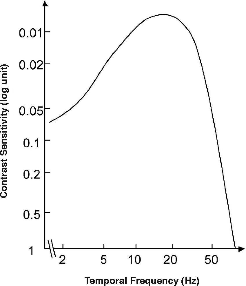
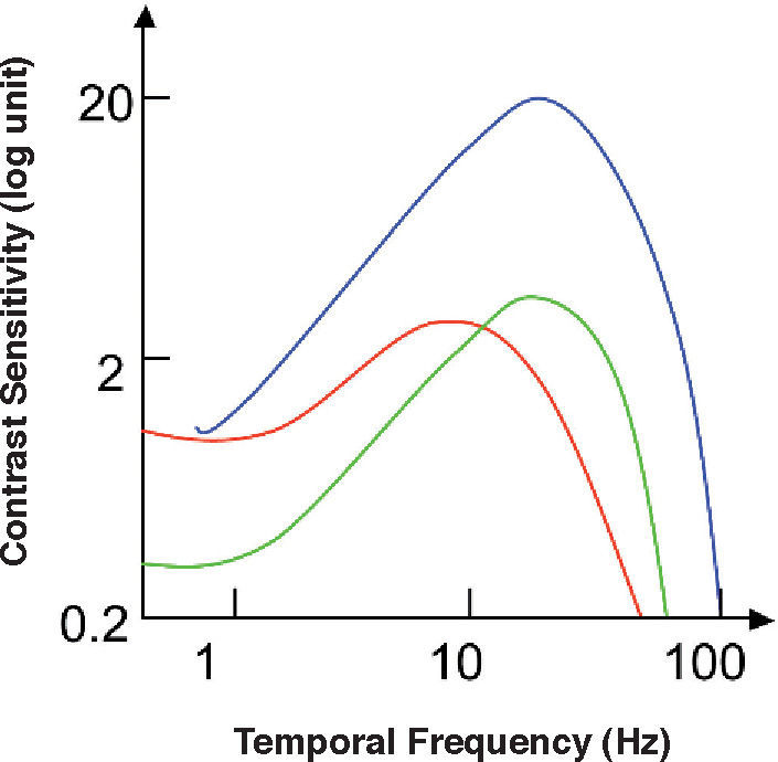
where ft is the temporal frequency and the meaning of the remaining parameters is the same as in Equation 2. Consequently, the definitions of contrast (Equation 5) and contrast sensitivity (Equation 8) we have introduced above also apply to this kind of stimuli, and the function relating contrast sensitivity to temporal frequency is called “temporal contrast sensitivity function” (in what follows, tCSF for short). The shape of the achromatic tCSF for a normal observer is similar to that of the spatial CSF: it is also bandpass shaped (Figure 12), although the low-frequency fall-off shows a characteristic concavity. At photopic levels, the peak frequency lies about 8-10 Hz. The temporal resolution, often called Critical Flicker Frequency (CFF) may even exceed 50 Hz under favourable conditions.

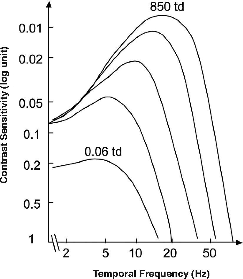
As happens with the spatial CSF, the tCSF also depends on a considerable number of factors, including luminance, spatial extent and eccentricity. The effect of mean luminance is shown in figure 13. The law governing sensitivity changes with mean luminance is Weber's in the low frequency region; however, at high frequencies it is the threshold amplitude that remains invariant with mean luminance; that is, the threshold contrast is inversely proportional to mean luminance.71-72 A classical related effect is the increase of the CFF with mean luminance (similar to the behaviour exhibited by visual acuity); this effect is known as the Ferry-Porter law [see, for example, the chapter by N. J. Coletta in Norton et al.’s book73].
 to high retinal illuminance (top: 850 td)")
Dependence of the temporal CSF on the state of adaptation (from low (bottom: 0.06 td) to high retinal illuminance (top: 850 td)
Increasing the size of the stimulus increases contrast sensitivity at any given frequency, while maintaining the maximum of the tCSF at the same frequency value.74 As a consequence, the CFF increases with size.75 The tCSF decreases globally with increasing eccentricity, although again the maximum does not change its position.76 However, unlike visual acuity, higher CFF values are found outside the fovea at scotopic levels.77
Contrast Sensitivity in the Spatio-temporal DomainA luminance pattern that changes as a function of position (x, y) and time is a spatio-temporal pattern. Spatio-temporal patterns usually employed as stimuli in visual research are counterphase gratings and travelling gratings. In counterphase sine gratings luminance is sinusoidally modulated both in space (with frequencies fx, fy) and in time (with frequency ft), If, in particular, fy=0, the corresponding luminance profile would be:
A travelling grating is a spatial pattern that moves with a given velocity, v. If we assume fy=0, the luminance profile would be:
where ft= v x fx is the temporal frequency of the luminance modulation caused by the motion at each point (x,y) of the pattern, and the sign (±) accompanying the variable v indicates whether the grating is moving towards the left or the right, respectively.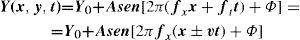
The usual definitions of contrast and contrast sensibility also apply to these patterns, but contrast sensitivity becomes here a 3D function, or 2D if the spatial pattern is 1D, that is, if the modulation occurs only along the x or the y directions. In what follows, we will refer to that function as the “spatio-temporal CSF”.
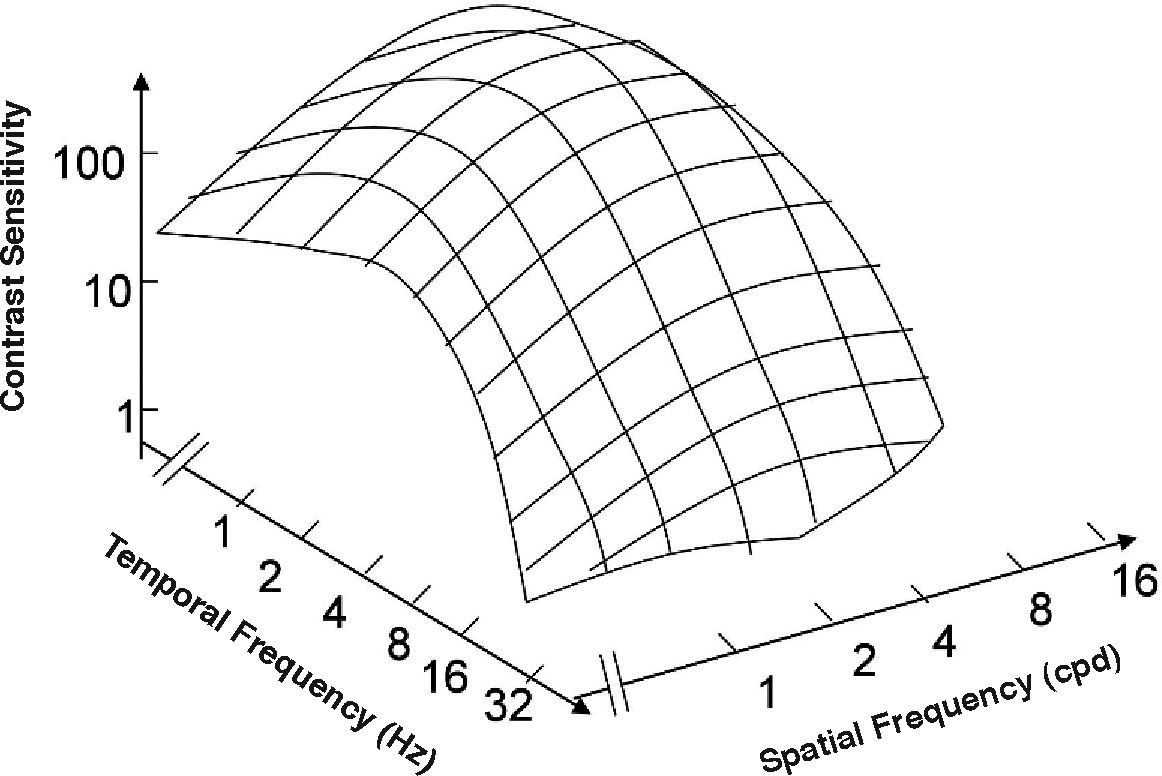
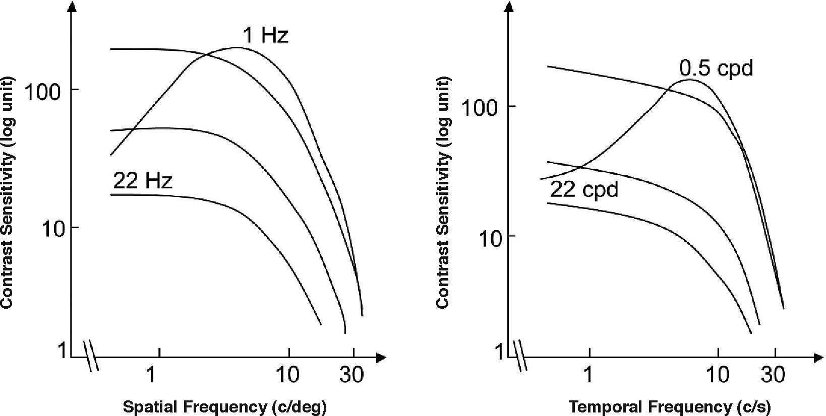
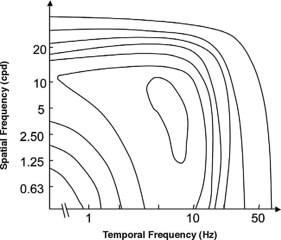
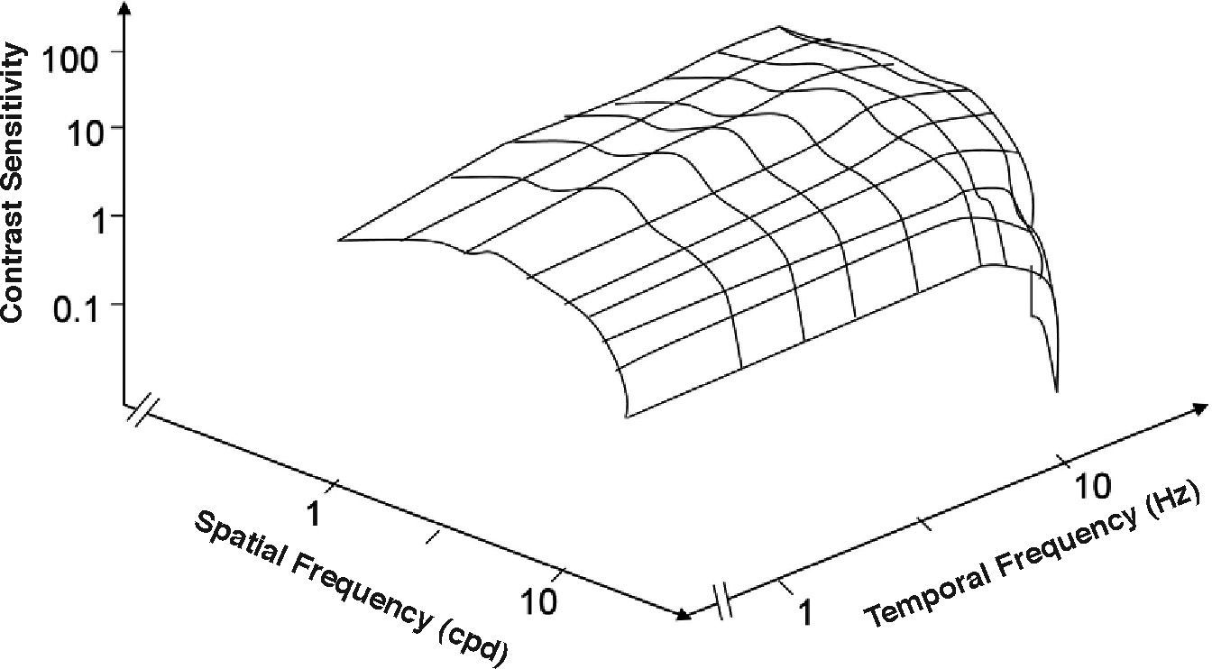
The spatio-temporal CSF (Figure 14) is a band-pass surface.78 If cross-sections of the 2D surface are performed for different spatial frequencies or temporal frequency planes, the spatial and temporal CSFs plotted in figure 15 are obtained. The shape of the spatial CSF changes from band pass to low pass with increasing temporal frequency, and the same happens to the temporal CSF when the spatial frequency increases. Besides, the spatial resolution decreases with increasing temporal frequency, while the temporal resolution decreases with increasing spatial frequency. Although the curves shown here were obtained with square gratings,79 basically the same behaviour is found with sinusoidal gratings. The geometrical locus of (fx,ft) points for which detection only occurs at unit contrast defines what is known as the spatio-temporal visibility window (see Figure 16). The appearance of a counterphased grating at and above threshold depends on its exact location within the visibility window. In fact, only when the temporal frequency is particularly low (less than 1 Hz), the pattern is perceived as flickering. When the spatial frequency is particularly low (below 0.5 cpd) and the temporal frequency is high enough, the apparent spatial frequency of the gratings is twice its nominal value.80 This effect is known as “frequency doubling” and the device known as FDT is named after this phenomenon. Within the rest of the visibility window (and therefore, within its greater extent) apparent motion is seen, and the probability of its being perceived towards the left or the right is the same [see, for example, the chapter by D. Burr in J. Kulikowski et al.’s book81].

The spatio-temporal CSF surface It is bandpass, with a maximum in the 3-4 cpd region with 8-10 Hz.
 or the spatial temporal frequency (right), to obtain, respectively, the spatial and the temporal CSFs.")
Cross-sections of the 2D spatio-temporal CSF surface at different values of the temporal (left) or the spatial temporal frequency (right), to obtain, respectively, the spatial and the temporal CSFs.

Contours of constant contrast sensitivity. The outer boundary represents the spatio-temporal window of visibility.
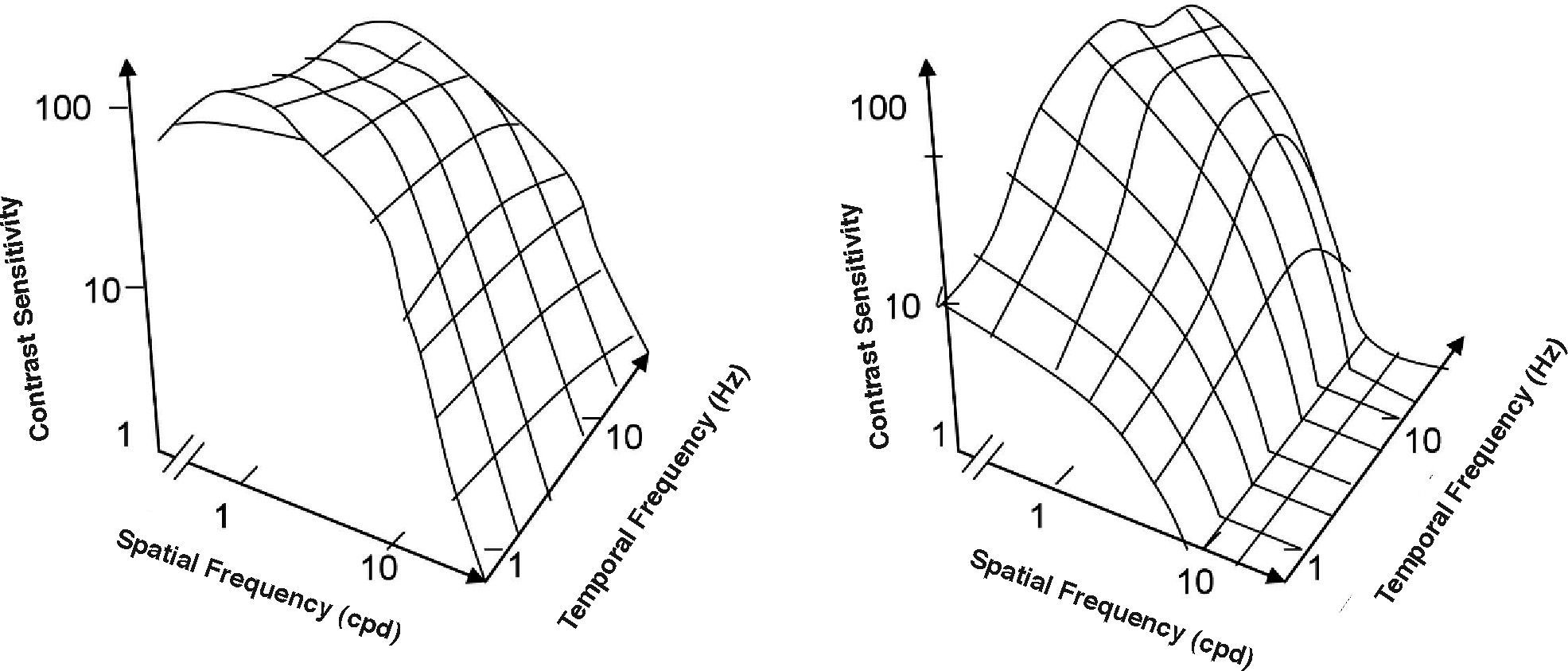
Obviously, the 2D spatio-temporal CSF may be considered as the envelope of two surfaces, one of them being the CSF measured after selectively destroying the magnocellular system (Figure 17, left) and the other being the CSF obtained after selectively destroying the parvocellular system (Figure 17, right). Experiments carried out with monkeys show that the shape of the spatio-temporal CSF matches the Parvo-only surface, excluding the low spatial-high temporal frequency corner, meaning that, except for that region, detection of spatio-temporal sinusoidal patterns is mediated by the parvocellular pathway.82,83 There is a reasonably good match between the characteristics of the psychophysical Parvo-only surface and the CSFs of individual Parvo cells (Figure 18). 84,85 One must be careful, however, about what is meant by “low-spatial and high-temporal frequency region”. Note that if cross-sections of the Magno-only and Parvo-only surfaces are taken at a sufficiently low spatial frequency (at least, for values up to 0.5 cpd), it can be seen that the Magno tCSF is higher than the Parvo one, provided that the temporal frequency is above a not-particularly-high value (about 2 or 3 Hz; see Figure 6, right). Note that this behaviour is not entirely consistent with the properties of individual cells. In fact, individual M cells are more sensitive to stationary gratings than P cells, provided that the spatial frequency is not to high (as we have seen above) and, besides, this happens also for values of the temporal frequency that are not particularly high, provided that the spatial frequency is low enough. It is true, however, that the global properties of a mechanism do not depend only on the properties of its individual components, but also on the way those components interact.
 and the parvocellular systems (right) in a macaque monkey.")
CSF surfaces measured after selectively destroying the magnocellular (left) and the parvocellular systems (right) in a macaque monkey.

CSF surface of a Parvo cell. There is a reasonably good match between the characteristics of this surface and those of the psychophysical Parvo-only surface of Figure 18.
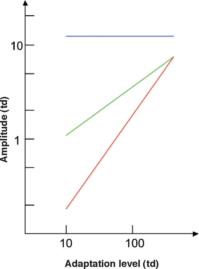
The spatial and temporal frequencies of the pattern determine the dependence of contrast sensitivity on adaptation state (Figure 19). Weber's law holds true if both frequencies are particularly low, but the regime changes to DeVries-Rose's law at high spatial and low temporal frequencies, while the amplitude threshold remains independent of the mean luminance at high temporal and low spatial frequencies. The extent of the regions in the spatial domain governed by each of these three laws depends on the luminance range under evaluation.78
, green line is DeVries-Rose's law (holds at high spatial and low temporal frequencies), and blue line is the linear zone independent of mean luminance (holds at high temporal and low spatial frequencies)")
Dependence of the amplitude thresholds on the adaptation state for three different spatio-temporal stimuli. Red line is Weber's law (holds if both spatial and temporal frequencies are low), green line is DeVries-Rose's law (holds at high spatial and low temporal frequencies), and blue line is the linear zone independent of mean luminance (holds at high temporal and low spatial frequencies)
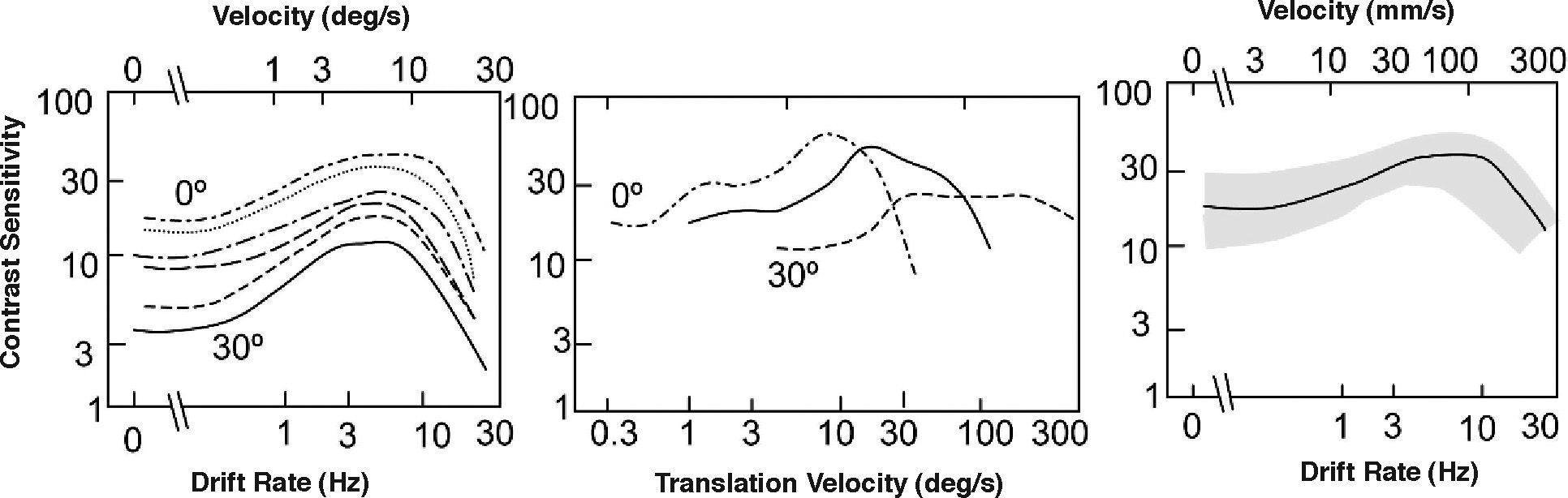
The same dependences with eccentricity shown above for the spatial CSF are observed, for any given frequency, when the gratings are also time-modulated. If contrast sensitivity is measured with gratings of fixed spatial frequency and varying temporal frequency, and the result are plotted as a function of temporal frequency, the overall sensitivity decreases with increasing eccentricity, although the shape of the curve does not change otherwise (Figure 20, left). However, if stimuli are scaled according to the cortical magnification factor and the sensitivities are plotted as a function of velocity, the peak sensitivity shifts towards progressively higher velocities as eccentricity increases (Figure 20, centre), but all curves collapse to a single one if velocity is measured in mm of cortex per second instead of degrees per second (Figure 20, right).76 It follows, therefore, that the visual cortex is not just spatially homogeneous, but is also homogeneous in the spatio-temporal domain: a single spatio-temporal CSF characterizes the behaviour of the whole cortex.
. Center and right figure show contrast sensitivity data as a function of the velocity of the grating obtained with stimuli that have been scaled by the cortical magnification factor for three eccentricities (left: 0°, right: 30°). In the central figure, velocity is measured in degrees per second and in the figure on the right-hand side it is given in millimetres of cortex per second.")
Temporal contrast sensitivity for a low spatial frequency as a function of temporal frequency, velocitiy and eccentricity. The figure on the left-hand side shows the tCSFs at different eccentricities (top: 0°, bottom: 30°). Center and right figure show contrast sensitivity data as a function of the velocity of the grating obtained with stimuli that have been scaled by the cortical magnification factor for three eccentricities (left: 0°, right: 30°). In the central figure, velocity is measured in degrees per second and in the figure on the right-hand side it is given in millimetres of cortex per second.
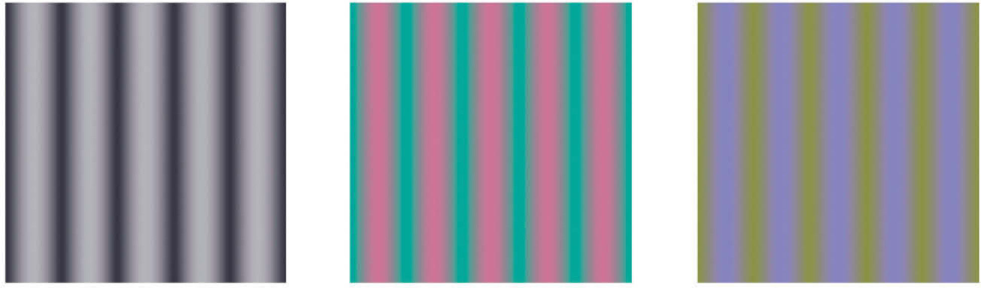
A spatial chromatic grating is a pattern where chromaticity changes with the spatial location, with a period defined by the spatial frequency fx. The profile of the spatial variation, as mentioned above, may be of different kinds, although it is usually sinusoidal and only occasionally square. Unless we explicitly state the contrary, we will only refer in what follows to experiments carried out with sinusoidal gratings. The truly relevant requirement that these patterns must fulfill is that the spatial changes have to be purely chromatic, that is, no clue for detection by an achromatic mechanism must be present. In general, a sinusoidal pattern with a colour palette confined to a given direction of colour space (or opponent modulation space)83 defined by the stimulus vector [ΔAS, ΔTS, ΔDS], has the form:
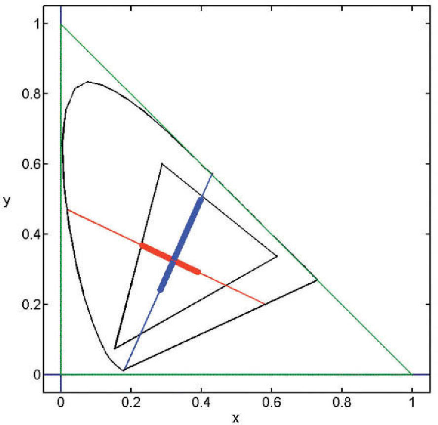
where ΔAS, ΔTS, ΔDS are the maximum response variations (or amplitudes) elicited by the pattern in the achromatic (A), red-green (T) and blue-yellow (D), mechanisms, measured from the mean response value in each mechanism. Note that the absolute value of this response is irrelevant to the discussion. The study of the exact nature of each of these mechanisms is outside the scope of this review, but the reader may assume that the achromatic mechanism is physiologically mediated by the magnocellular pathway, whereas T and D are mediated, respectively, by the parvo and koniocellular pathways. The interested reader may refer to the literature specialized in colour vision. The directions of colour space isolating a single mechanism (i.e. two of the components of the stimulus-vector are zero) are called cardinal directions.86 The cardinal directions of the chromatic mechanisms, plotted in the CIE1931 chroma-ticity diagram, are shown in figure 21. An example of the appearance of the gratings along such directions is shown in figure 22 (with fy=0). The limits that the reproduction device—a CRT monitor—sets on the colour palettes of these images appear in figure 21.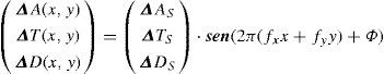

. Left: achromatic cardinal direction (A). Center: red-green cardinal direction (T). Right: blue-yellow cardinal direction (D).")
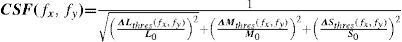
Contrast sensitivity in the colour space may be defined from the modulus of the stimulus vector at detection threshold as:
where [ΔAthres, ΔTthres, ΔDthres] = kthres[ΔAs, ΔTs, ΔDs] is the vector in the direction defined by the stimulus vector and with a modulus that just allowing allows for the pattern to be detected.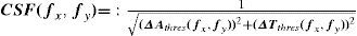
Alternatively, patterns like those defined by Equation 16 may also be described in the so-called “cone contrast space” by a vector containing the contrasts the stimulus produces in the three cone classes, that is, ΔLSL0,ΔMSM0,ΔSSS0where ΔLS, ΔMS, ΔSS are the maximum response variations (or amplitudes) elicited by the pattern in the three cone types, and measured from the mean response value in each cone type, L0, M0 and S0. The modulus of this vector is called “global cone contrast of the stimulus”. Assuming some properties for the mechanisms, it can be easily demonstrated that the relation between the amplitude of the responses in the mechanisms A, T, D and the amplitude of the responses in the cones L, M, S, is given by;
where Ka, Kt, Kdare scaling constants defining unit response in each mechanism. If these constants are chosen so that a stimulus isolating a mechanism and producing a global cone contrast of one, yields a unit response in the isolated mechanism,87 we are provided with a common metric for the three cardinal directions of colour space, which would allow us to compare thresholds measured along these directions. This representation space was originally proposed by Derrington, Krauskopf and Lennie, and is usually known as the DKL space or “opponent modulation space”.88 For an elegant mathematical treatment of this space, including a detailed discussion of the properties assumed for the mechanisms, the reader may refer to the tutorial by D. H. Brainard in Kaiser and Boynton's book.89 However, another procedure is possible. The reciprocal equation:yields the cone contrasts generated by the stimulus, from which the contrast sensitivity may be calculated as the inverse of the global cone contrast at detection threshold, i.e.: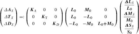
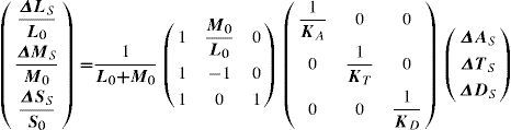
This definition improves the one given by Equation (17) because, as it uses a common metric for all stimuli, thresholds along any direction of the colour space (and not only along the three cardinal ones) can be compared. The chromatic contrast sensitivity functions (cCSFs) are low-pass, that is, the maximum sensitivity is reached when the spatial frequency tends towards zero, as can be seen in figure 23. At any frequency, sensitivity measured with red-green gratings is higher than that obtained with blue-yellow gratings and, therefore, spatial resolution with red-green gratings is also higher than that obtained with blue-yellow ones (values of the cutoff frequency are around 12 and 10 cpd, respectively). As can also be seen in figure 23, red-green and blue-yellow sensitivities are higher than achromatic sensitivity for particularly low spatial frequencies (lower than 0.5 cpd).90-91 (Valverg A, et al. IOVS. 1997;38:S893). When determining the blue-yellow CSF, chromatic aberration must be eliminated, or otherwise the grating shall be distorted by achromatic artefacts, which would increase the probability of detections by an achromatic mechanism, a circumstance that must be avoided. The effect of chromatic aberration, however, is important only for spatial frequencies above 3-4 cpd.92
 for the A, T and D isolated mechanisms.")
Chromatic and achromatic sensitivities are affected basically by the same factors, although they do not necessarily follow the same laws. For instance, the transition between the De Vries-Rose's and Weber's laws occurs at a luminance level that depends on spatial frequency, but this dependence is not the same for chromatic and for achromatic gratings.50,93-94
Literature on the variation of chromatic sensitivity with eccentricity is scarce. It is known, however, that the peak sensitivity to red-green gratings decreases much faster with eccentricity than that observed with blue-yellow gratings, in significant agreement with the rate at which P and K densities decreases. If sensitivity drops are examined in comparable conditions—meaning that for each direction in the colour space the optimal spatial frequency must be used—the sensitivity attenuation rates for the blue-yellow and for the achromatic mechanisms are comparable.95
Chromatic Contrast Sensitivity in the Spatio-temporal DomainChromatic contrast in a spatially uniform stimulus may be sinusoidally time-modulated along any direction of the colour space, in such a way that the following equation will hold in any point of the stimulus:
where ft is the temporal frequency. The remaining parameters have the same meaning as in Equation 16.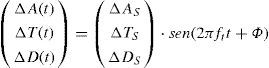
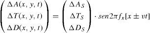
It is also possible to generate patterns that are simultaneously modulated in space and time, governed either by the following equation:
or, if a travelling grating is preferred:where we have assumed, for simplicity's sake, that fy=0.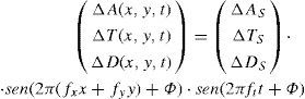
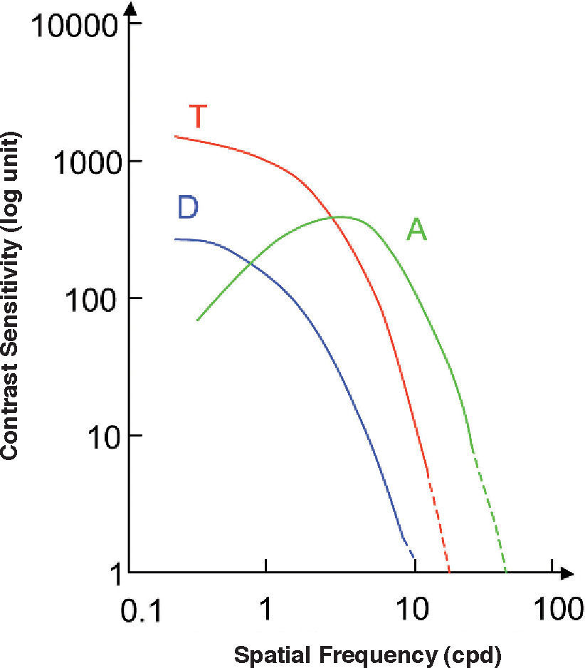
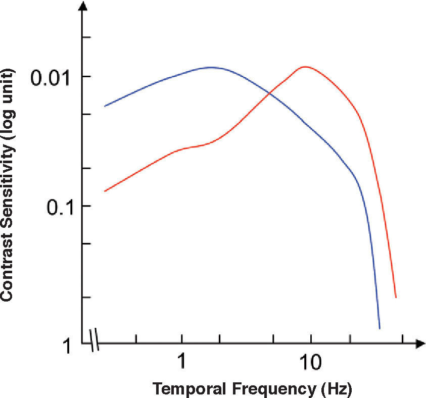
The chromatic temporal contrast sensitivity function (ctCSF) is also basically low-pass, although with a slight attenuation at low frequencies, as shown in figure 24.72,96-98 Such attenuation is also present in the temporal chromatic CSFs of any individual Parvo cell (Figure 25), but its magnitude is far lower than the low-frequency attenuation found in the achromatic CSF of the same cell (Figure 25) and, of course, it is negligible in comparison with that found in the CSF of a Magno cell (Figure 25).99 At present, a mass of evidence supports the idea that the detection of temporal achromatic and chromatic (red-green) patterns is mediated, respectively, by the magnocellular and parvoce-llular pathways.100-103
 and achromatic (red curve) temporal contrast sensitivity functions.")
Red-green (blue curve) and achromatic (red curve) temporal contrast sensitivity functions.
 and achromatic (green line) temporal contrast sensitivity functions for a Parvo cell and achromatic temporal sensitivity function for a Magno cell (blue line).")
Red-green (red line) and achromatic (green line) temporal contrast sensitivity functions for a Parvo cell and achromatic temporal sensitivity function for a Magno cell (blue line).
Temporal chromatic gratings modulated along the cardinal direction of the red-green mechanism contain achromatic artefacts due to latency differences between the L and M cone responses that constitute the input of the opponent Parvo cells.104 If this effect is not compensated—which is not a trivial thing, given that the effect depends on temporal frequency—the observer's sensitivity will be greater in a task consisting in detecting the temporal pattern than in a task consisting in detecting the chromatic pattern—i.e., the temporal pattern caused by colour differences—, since the observer detects a residual achromatic flicker even when the chromaticity of the test appears to be stationary.97 In particular, two different CFFs may be measured, one for flicker fusion (at about 20 Hz for a medium photopic level) and other for color fusion (which does hardly reach 10 Hz).
The influence of mean luminance on the chromatic tCSF is complex. Within a wide luminance range, contrast sensitivity increases with luminance in all the frequency spectrum. However, above a certain luminance level, the rate of increase is significantly higher (i.e., a faster increase) at high than at low spatial frequencies, a notch appears around 10 Hz and the shape of the CSF changes from low-pass to band-pass. All these effects point toward some kind of contribution from the magnocellular pathway to the detection of chromatic gratings.72 Since both the spatial and the temporal chromatic CSF are low-pass, it is not surprising that the spatio-temporal CSF is also low-pass shaped.105 There is not any paper in the literature about these kinds of measurements outside the fovea.
Additional Comments and some Suggestions for the UsersAs we commented in the Introduction, it is important to realise that relying on a single test as a method for early detection of a given pathology may prove not to be particularly useful. Actually, a test battery would be preferable, including at least a test that is selective for each of the physiological pathways (Magno, Parvo and Konio). In the literature, many examples are found where comparisons between different mechanism-selective tests are carried out—perimetries with different stimuli, for example—but those tests differ in the experimental task set to the patient and in the magnitude that is evaluated. For instance, in order to isolate the Magno pathway, FDT perimetry is used; to isolate the Parvo, high resolution perimetry would be adequate; and the Konio can be isolated by means of SWAP perimetry. In the first case it is contrast sensitivity that is measured; in the second it is spatial resolution and in the third one it is an incremental threshold that is measured. Deciding which of the three mechanisms under assessment is damaged to a greater extent is not trivial when a common metric is not available. In our view, one such metric could be contrast sensitivity. We suggest that by extending contrast sensitivity measurements outside the fovea, with patterns modulated along directions isolating, as far as possible, the achromatic, red-green and blue-yellow mechanisms, and with a sufficient sampling of the spatio-temporal frequency domain (a sampling whose limits and density ought to be discussed), the performance of this kind of measurements would significantly improve.
Taking into account how the different parameters of the stimuli influence contrast sensitivity, to ensure that the results of different experiments can be compared, they should be carried out obviously under a fixed set of conditions. The choice of those particular conditions should reduce the possibility of undesired alterations: e.g., those due to uncontrolled variation of the stimuli, or the possibility of intrusion of an undesired mechanism. For instance, it is preferable to work at a photopic level, because if for any reason this level changes—due, for example, to natural wear of the illumination source or to a cataract of the patient—the effect of the results will be smaller than when working at mesopic or scotopic levels. Following in the same line, stimuli ought to contain a sufficient number of cycles (at least 2.5) for all frequencies. On the other hand, given that the use of stimuli of fixed size would limit the extent of the visual field that can be analysed, since sensitivity would fall steeply with increasing eccentricity, measurements outside the fovea ought to be carried out after adapting, at each location, the stimulus size to the receptive field size. Finally, to avoid the intrusion of undesired mechanisms, the distorting effect of the stimulus border ought to be minimized (the border ought to be smoothed, by means of a Gaussian function, for instance), and the chromatic gratings used ought to be isoluminant patterns (ΔA=0) and modulated along the cardinal direction of the chromatic mechanism we want to isolate. If possible, the isoluminant condition ought to be determined for each patient to avoid the presence of (individual) achromatic artefacts. If this is the case, the cardinal directions of the chromatic mechanisms would correspond to patterns with the condition ΔT=0 (or ΔD=0), and the required value for ΔA.
At this point, one may wonder whether this kind of measurements is in practice more or less useful for clinical diagnosis. We are dealing with tests that, for different reasons, are hard to integrate in the routine test that are administered to all patients. For instance, they are time-consuming: the time required may be more than the practitioner can afford or may seem too long for the benefit the patient may ultimately get or may even put the endurance of the patient to a severe test, particularly with elderly subjects. Besides, many patients find it hard to understand the task that is set to them: they must be provided with careful instructions. And most important, the relatively large dispersion of the results makes diagnosis not a trivial thing. For all this reasons, it is tempting to believe that this kind of psychophysical measurements are better avoided and that structural measurements provide all we need to know. This is a point of view we do not share. We have recently presented preliminary results showing that subjects with normal optic disc retinography and optical coherence tomography (OCT) results, present significant alterations of their visual field (in comparison with an average normal observer of the same age range) if contrast sensitivity is measured for stimuli of adequate spatial and temporal frequency isolating the adequate color mechanism (Morilla-Grasa A. et al., 2009 ARVO E Abstract-5290/A220). Therefore, at least in certain cases, for us it seems difficult to question the usefulness of contrast sensitivity measurements in the spatio-temporal domain.
None of the authors has a financial or proprietary interest in any material or method mentioned in this report.
If stimuli were adapted in size to their frequency, that is, if they contain a fixed and sufficient number of cycles, the CSF measured at fovea and at eccentricity E would still exhibit the behaviour described above, and the general shape of the curves would not differ essentially from those in figure 9.


