

To evaluate the correlation between automated achromatic perimetry (AAP) and the output of two retinal nerve fiber layer (RNFL) analysers: scanning laser polarimetry (GDx-VCC) and optical coherence tomography (OCT).
MethodsQuantitative RNFL measurements with GDx-VCC and Stratus-OCT were obtained in one eye from 52 healthy subjects, 38 ocular hypertensive (OHT) patients and 94 glaucomatous patients. All patients underwent a complete examination, including AAP using the Swedish interactive threshold algorithm (SITA). The relationship between RNFL measurements and SITA visual field global indices were assessed by means of the following methods: analysis of variance, bivariate Pearson's correlation coefficient, multivariate linear regression techniques and nonlinear regression models, and the coefficient of determination (r2) was calculated.
ResultsRNFL thickness values were significantly lower in glaucomatous eyes than in healthy and ocular hypertensive eyes for both nerve fiber analysers (P≤0.001), except for the inferior 120° average thickness in GDx-VCC. Linear regression models constructed for GDx-VCC measurements and OCT-derived RNFL thickness with SITA visual field global indices demonstrated that, for the mean deviation, the only predictor in the model was the nerve fiber indicator for GDx-VCC (r2=0.255), and for the pattern standard deviation, the predictors in the model were the nerve fiber indicator for GDx-VCC (r2=0.246) and the maximum thickness in the superior quadrant for Stratus-OCT (r2=0.196). The best curvilinear fit was obtained with the cubic model.
ConclusionsQuantitative measurements of RNFL thickness using either GDx-VCC or OCT correlate moderately with visual field global indices in moderate glaucoma patients. We did not find a correlation between visual field global indices and RNFL thickness in early glaucoma patients. Further study is needed to develop new analytical methods that will increase RNFL analyser's sensitivity in early glaucoma patients.
Evaluar la correlación entre la perimetría automatizada acromática (PAA) y la medida obtenida con dos dispositivos analizadores de la capa de fibras nerviosas de la retina (CFNR): el polarímetro láser de barrido (GDx-VCC) y el tomógrafo de coherencia óptica (Stratus-OCT).
MétodosSe realizaron medidas cuantitativas de la CFNR utilizando los dispositivos GDx-VCC y el Stratus-OCT en un ojo de 52 sujetos sanos, 38 pacientes con hipertensión ocular (HTO) y 94 pacientes glaucomatosos. A todos los pacientes se les realizó una exploración completa, que incluyó medidas de PAA utilizando el algoritmo sueco de umbral interactivo (SITA, en inglés). Se estudió la relación entre las medidas de la CFNR y los índices globales SITA del campo visual utilizando para ello los siguientes tipos de análisis estadístico: análisis de la varianza, coeficiente de correlación de Pearson bivariante, técnicas de regresión lineal múltiple (multivariante) y modelos de regresión no lineales, calculándose el coeficiente de determinación (r2).
ResultadosPara ambos analizadores de las fibras nerviosas, los valores medidos del espesor de la CFNR resultaron ser significativamente menores (P≤0,001) en ojos glaucomatosos que en ojos sanos o con hipertensión ocular, a excepción de los resultados obtenidos con el GDx-VCC para el espesor promedio del sector inferior de 120°. Los modelos de regresión lineal elaborados para comparar las medidas del espesor de la CFNR (obtenidas con el GDx-VCC y con el Stratus-OCT) con los índices globales SITA del campo visual pusieron de manifiesto que, para la desviación media, la única variable predictora aceptable en el modelo fue el indicador de fibras nerviosas para el GDx-VCC (r2=0,255), y en lo que respecta a la desviación típica del patrón, las variables predictoras del modelo fueron el indicador de fibras nerviosas para el GDx-VCC (r2=0,246) y el espesor máximo en el cuadrante superior en el caso del Stratus-OCT (r2=0,196). El mejor ajuste curvilíneo se obtuvo con el modelo cúbico.
ConclusionesLas medidas cuantitativas del espesor de la CFNR utilizando bien el GDx-VCC o dispositivos basados en la tomografía de coherencia óptica están correlacionadas de forma moderada con los índices globales del campo visual en pacientes con glaucoma. Sin embargo, no hallamos una correlación entre los índices globales del campo visual y el espesor de la CFNR en aquellos pacientes con glaucoma incipiente. Es necesario proseguir con la investigación para desarrollar nuevos métodos analíticos que aumenten la sensibilidad de los analizadores de la CFNR en aquellos pacientes con glaucoma incipiente o en fase inicial.
Glaucoma is a progressive optic neuropathy characterized by structural changes of the optic nerve that are associated with the development of functional visual defects.1 Detection of glaucomatous damage is possible through observation of the optic nerve head (ONH) and the retinal nerve fiber layer (RNFL) and through the measurement of the visual function with automated achromatic perimetry (AAP).2,3 However, both the subjective observation of optic disc changes and the results of automated perimetry are prone to variability4, and the efficacy of AAP in glaucoma is somewhat limited by the subjective nature of the patient's response.5
Recent advances in ocular imaging technology using different optical properties of the RNFL provide a quantitative way to assess optic disc topography and/or the thickness of the RNFL thickness.6 Both scanning laser polarimetry (SLP) and optical coherence tomography (OCT) can provide objective and reproducible measures of RNFL thickness,7-10 and a significant correlation has been observed between Stratus OCT and GDx-VCC RNFL measurements.11 Both instruments are being increasingly used in the clinical practice, because previous studies have shown a significant correlation between OCT and GDx-VCC in what concerns RNFL measurements and since they have revealed as being useful methods for objective detection and quantification of glaucomatous RNFL atrophy12,13.
A straightforward relationship between structure and function in the context of glaucoma has not been yet conclusively published in the scientific literature. However, quantitative measurements of ONH and RNFL thickness in early longitudinal studies have revealed as promising in detecting progressive glaucoma14 and in monitoring glaucomatous changes.15,16 For these technologies to be clinically relevant, they should be significantly correlated with other accepted techniques to determine glaucomatous optic nerve damage, the most usual of which is standard AAP.8
This prospective cross-sectional study was designed to test the relationship between the output of two RNFL analysers (the GDx-VCC and the Stratus-OCT) and the visual field global indices measured with AAP in normal subjects, ocular hypertensive (OHT) subjects and initial and moderate glaucomatous eyes. Moreover, different regression models will be applied in order to investigate which functions —linear or nonlinear— best describe structure-function associations between them. We believe that the relationship between the parameters yielded by GDx-VCC and OCT (in particular, superior and inferior RNFL thicknesses) should become increasingly stronger as the disease state worsens, and should prove to be useful to detect and monitor glaucoma patients.
MethodsSubjectsThis prospective, non-randomized, cross-sectional analysis of normal, OHT and glaucomatous eyes was carried out in 184 subjects (184 eyes). One eye from each of the 52 healthy (28.26%), 38 OHT (20.65%), 58 early glaucomatous (31.52%) and 36 moderate glaucomatous (19.56%) subjects was analysed. We did not include in the study normal-tension glaucoma patients. All the procedures were conducted in accordance with the principles of the Helsinki Declaration. Detailed consent forms were obtained from each of the patients.
All patients underwent a complete ophthalmic examination, which included systemic, ocular, and family history, best-corrected visual acuity by means of a standard Snellen projector system, slit-lamp biomicroscopy including gonioscopy; diurnal applanation tonometry measurement and stereoscopic optic disc evaluation using a 78-diopter lens (with cup/disc ratios assessed by the same experienced examiner). Achromatic visual field testing with SITA standard strategy were carried out using the Humphrey 750 Visual Field Analyser program 24-2 (Zeiss Humphrey Systems, San Leandro, CA, USA). SLP measurements were obtained with the GDx-VCC, software version 5.1.0 (Laser Diagnostic Technologies, San Diego, California, USA). OCT measurements were carried out using the Stratus-OCT, version 3.0 (Carl Zeiss Meditec Inc, Dublin, CA, USA).
Normal eyes were defined as those with intraocular pressure (IOP) not exceeding 21 mmHg and having no prior history of elevated IOP, reproducible normal visual field as measured with AAP [glaucoma hemifield test, mean deviation (MD) and pattern standard deviation (PSD) within normal limits] and a healthy optic nerve head (ONH) appearance (asymmetry of vertical cup/disc ratio <0.2, no evidence of rim thinning, notching, excavation, haemorrhage, or RNFL defects). OHT subjects had an IOP greater than 21 mmHg but reproducible normal visual fields with healthy ONH appearance. Glaucoma patients were defined as having either specific and repeatable glaucomatous achromatic visual field defects or clinical judgment of glaucomatous optic neuropathy (GON), based on the presence of at least one of the following characteristics that are indicative of glaucoma: cup-to-disc ratio asymmetry between fellow eyes greater than 0.2, cup excavation greater than 0.6, altered neuroretinal rim with focal or general thinning, peripapillary haemorrhages, notches, or localized pallor.
Exclusion criteria for all patients included: best-corrected visual acuity worse than 20/40, refractive error exceeding +/-5.00 dioptres of sphere or 2.00 dioptres of cylinder, evidence of vitreous or retinal pathology not attributed to glaucoma (including diabetic retinopathy, age-related macular degeneration, cystoid macular oedema and peripapillary atrophy extending to 1.7 mm from disk centre), advanced visual field loss (defined by defects close to fixation 5 dB below normal and/or an AGIS score > 11), unreliable AAP or other pathological conditions that could affect the visual field (pituitary lesions, demyelinating diseases), secondary causes of IOP increase (corticosteroid use, iridocyclitis, trauma) and prior incisional surgery or laser treatment.
Visual Field (VF) TestingAAP was performed with the Humphrey Field Analyser (Humphrey Systems Inc, Leandro, CA, USA) using the Swedish Interactive Threshold Algorithm (SITA) standard strategy, program 24-2 test procedure and a size-III stimulus. The analysis of the data was carried out by the program STATPAC 2, included in the software of the perimeter. All patients had undergone automated perimetry before.
Perimetry was performed within 3 months of clinical examination and determination of RNFL thickness. AAP reliability criteria to accept a VF examination as valid included: fixation-loss rates of less than 20% and maximum false-positive and false-negative rates of 25%. The unreliable VF examinations were rejected and repeated.
The criteria used to establish an abnormal visual field consisted of a specific and repeatable glaucomatous achromatic visual field defect that produced three or more significant (P<0.05) non-edge-contiguous points with at least one at P<0.01 on the same side of the horizontal meridian in the pattern deviation plot and classified outside normal limits in the Glaucoma Hemifield Test. Visual field (VF) defects were considered reproducible if they met the criteria for abnormality and were present in exactly the same field locations in at least one consecutive VF confirmatory examination.
The severity of the disease in the case of glaucomatous eyes was graded using the Advanced Glaucoma Intervention Study (AGIS) scores.17 The AGIS algorithm for scoring visual field defects is based on reliability, the number of adjacent test locations with depressed sensitivity, the depth of the depression, and the region of the field affected.18 In the present study, the stratification of glaucomatous field losses were classified according to the AGIS criteria as follows: early visual field damage (AGIS score < 6), moderate visual field damage (AGIS score between 6 and 11) and severe visual field damage (AGIS score > 11). Patients with severe visual field damage were not included in the study, in order to avoid truncation effects and their difficulty to undergo VF examinations.
Measures of VF depression presented on the Humphrey printout include the mean deviation (MD) and the pattern standard deviation (PSD). Therefore, MD will reflect generalised glaucomatous VF loss, while PSD will reflect small localised defects that would appear in early stages of glaucoma. As a result, MD will detect better a generalized glaucomatous VF loss than small localized defects that would appear in early stages of glaucoma; these ones will be better revealed using the PSD. The MD and PSD were used for the statistical analysis, in order to evaluate the correlation between RNFL structural measurements obtained with the RNFL analysers and the visual field global indices measured with AAP.
SLP: GDx-VCC MeasurementsWith the advent of SLP with Variable Corneal Compensation (GDx-VCC, Laser Diagnostic Technology, Inc., San Diego, CA, USA), an objective means of evaluating relative RNFL thickness has been developed, with automated individualized compensation of anterior segment birefringence. This technology uses a scanning laser to obtain images of the RNFL, from which it calculates the relative RNFL thickness. With SLP, linearly polarized light traversing the RNFL, which is presumably a birefringent medium, is elliptically polarized, and bounces back out of the retina. The amount of linear retardation of the light at each retinal location has been shown to be proportional to the corresponding RNFL thickness.7,8 This technology has been described in detail elsewhere.19-21
The GDx-VCC Nerve Fiber Layer Analyser is a commercially available scanning laser polarimeter, designed to estimate RNFL thickness “in vivo”. In our study, at each imaging session, a well trained operator performed all the RNFL thickness measurements. Three consecutive values of the RNFL thickness were obtained in each eye in an undilated state along the visual axis and central cornea. Only high-quality images that had passed the internal software's automated quality control criteria were accepted. Images that were obtained during eye movement, or unfocused and poorly centred images were rejected and taken again. Lastly, the optic disc margin was approximated by a circle or an ellipse placed by an experienced technician around the inner margin of the peripapillary scleral ring. Default quadrant positions (as supplied by the manufacturer) were applied: the peripapillary band was divided into superior and inferior segments of 120° each, a temporal segment of 50°, and a nasal segment of 70°.
OCT MeasurementsThe Zeiss Optical Coherence Tomography Model 3000 (Stratus-OCT; Humphrey Systems, Dublin, CA, USA) is a noncontact and noninvasive technology that allows crosssectional imaging of the human retina at histologic levels of resolution (approximately 10 μm), based on the principles of low-coherence interferometry.4,22 It is designed to provide real-time, objective, cross-sectional measurements of various layers of the retina, including the RNFL.2 A scanning interferometer is used to obtain a cross section of the retina based on the reflectivity of its different layers.8 A high reflectance layer located just under the inner surface of the retina that corresponds to the RNFL thickness is measured with a computer algorithm to give RNFL thickness.7,8 Detailed descriptions of the principles of OCT have already been published.23-25
Image acquisition was as follows: after pupillary dilation with 1% tropicamide to achieve a minimum diameter of 5 mm to maximize the likelihood of acquiring a high-quality image, the RNFL was scanned with the Stratus-OCT. Three circular scans of 3.4 mm diameter centred on the optic disc, judged to be of acceptable quality by an experienced observer, were obtained and stored for each eye tested. The scan process was started and the image of the ONH was focused and aligned using the real time video monitor. When the operator was satisfied with the focus and quality of the scan image, it was frozen and saved in a database. RNFL thickness is quantified by an automated computer algorithm that identifies the anterior and posterior borders of the RNFL. The data are presented by clock hours, by quadrants, and overall.
Statistical AnalysisQuantitative variables were compared using the one-way analysis of variance (ANOVA) to evaluate different measures among the groups. Results of statistical significance were also provided after Bonferroni correction based on the number of comparisons within each analysis, in order to determine which pairs of means differ, as reflected in the correlation tables. Prior to the use of parametric tests, the variables under study (data from AAP, GDx-VCC or OCT) were confirmed to behave as normal variables in any of the examinations performed by means of Kolmogorov-Smirnov test, and homogeneity in group variances were contrasted.
Statistical correlations between parameters were assessed using the bivariate Pearson's correlation coefficient, multivariate linear regression techniques and nonlinear regression models. Different nonlinear regression models for curve estimation were used and compared: logarithmic, inverse, quadratic, cubic, power, compound, S-curve, and logistic. The coefficient of determination (r2) was calculated. A P-value less than or equal to 0.05 was considered to be statistically significant.
One eye was used from each subject for the statistical analysis. For healthy and OHT subjects the eye was randomly selected. For the data to be as unbiased as possible, in glaucoma patients the selected eye was the worst one, since some glaucoma subjects only had one damaged eye. By choosing a random eye from these subjects, there would be a significant proportion of healthy eyes from glaucomatous subjects included in the glaucoma group, which would inevitably affect the results.
Five parameters generated by the Nerve Fiber Analyzer (NFA) available mapping software were selected from each instrument for the statistical analysis. In the SLP GDx-VCC, we evaluated the following: the calculation circle average thickness (TSNIT), the superior 120° average thickness (SAVG), the inferior 120° average thickness (IAVG), the calculation circle standard deviation (TSNIT SD) and the nerve fiber indicator (NFI). The first three are average-based parameters, the fourth is a ratio-based parameter and the fifth is a constructed retardation parameter. These five parameters were selected for the statistical analysis because they have proven to be more sensitive than those presented in the TSNIT parameters table.26 With the Stratus-OCT we evaluated the maximum thickness in the superior quadrant (SMAX), the maximum thickness in the inferior quadrant (IMAX), the average thickness in the superior quadrant (AVGSQ), the average thickness in the inferior quadrant (AVGIQ) and the average thickness for the total circumference (AVGT). These five parameters were considered because they provide a quantitative evaluation of the thickness of the peripapillary retinal nerve fiber layer (which is useful to assess current or progressive glaucoma damage) and since they are probably the most relevant ones to the clinical community.
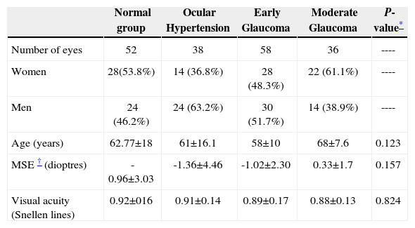
ResultsTable 1 summarizes the basic demographic characteristics of the study's population. There were no significant differences among the groups with regard to age, gender, or refraction.
Demographics and clinical data of the population under study, for each of the four groups (expressed as number of subjects, percentage and mean ± standard deviation)
| Normal group | Ocular Hypertension | Early Glaucoma | Moderate Glaucoma | P-value* | |
| Number of eyes | 52 | 38 | 58 | 36 | ---- |
| Women | 28(53.8%) | 14 (36.8%) | 28 (48.3%) | 22 (61.1%) | ---- |
| Men | 24 (46.2%) | 24 (63.2%) | 30 (51.7%) | 14 (38.9%) | ---- |
| Age (years) | 62.77±18 | 61±16.1 | 58±10 | 68±7.6 | 0.123 |
| MSE † (dioptres) | -0.96±3.03 | -1.36±4.46 | -1.02±2.30 | 0.33±1.7 | 0.157 |
| Visual acuity (Snellen lines) | 0.92±016 | 0.91±0.14 | 0.89±0.17 | 0.88±0.13 | 0.824 |
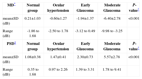
All normal and OHT eyes had normal achromatic visual fields. Patients with glaucoma had average automated perimetry values -MD and PSD- that were significantly different from those obtained for normal and OHT subjects. Table 2 displays a summary of these data.
Descriptive statistics of Visual Field Global Indices
| MD* | Normal group | Ocular hypertension | Early Glaucoma | Moderate Glaucoma | P-value† |
| mean±SD (dB) | 0.21±1.03 | -0.60±1.27 | -1.94±1.37 | -6.40±2.78 | <0.001 |
| Range (dB) | -1.86 to 1.68 | -2.50 to 1.78 | -3.12 to 0.49 | -9.98 to -3.25 | |
| PSD‡ | Normal group | Ocular hypertension | Early Glaucoma | Moderate Glaucoma | P-value† |
| mean±SD (dB) | 1.08±0.38 | 1.47±0.41 | 2.30±0.73 | 5.57±2.78 | <0.001 |
| Range (dB) | 0.35 to 1.68 | 0.97 to 2.26 | 1.39 to 3.31 | 1.78 to 9.41 |
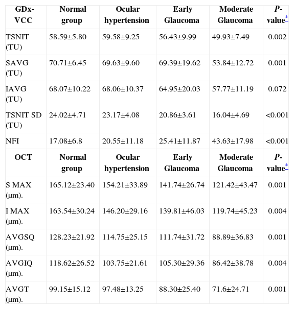
As illustrated in table 3, both nerve fiber analysers could differentiate normal and OHT eyes from eyes with glaucoma. For GDx-VCC, four parameters revealed statistically significant differences in the one-way ANOVA analysis for all patients: TSNIT, SAVG, TSNIT SD and NFI. Mean RNFL thickness measured with Stratus-OCT was significantly lower in glaucomatous eyes than in OHT and normal eyes. However, considerable measurement overlap at the means and standard deviations for both instruments were observed among normal, ocular hypertensive, and early glaucomatous eyes.
Descriptive statistics of the RNFL Analyser Parameters (mean±SD)
| GDx-VCC | Normal group | Ocular hypertension | Early Glaucoma | Moderate Glaucoma | P-value* |
| TSNIT (TU) | 58.59±5.80 | 59.58±9.25 | 56.43±9.99 | 49.93±7.49 | 0.002 |
| SAVG (TU) | 70.71±6.45 | 69.63±9.60 | 69.39±19.62 | 53.84±12.72 | 0.001 |
| IAVG (TU) | 68.07±10.22 | 68.06±10.37 | 64.95±20.03 | 57.77±11.19 | 0.072 |
| TSNIT SD (TU) | 24.02±4.71 | 23.17±4.08 | 20.86±3.61 | 16.04±4.69 | <0.001 |
| NFI | 17.08±6.8 | 20.55±11.18 | 25.41±11.87 | 43.63±17.98 | <0.001 |
| OCT | Normal group | Ocular hypertension | Early Glaucoma | Moderate Glaucoma | P-value* |
| S MAX (μm). | 165.12±23.40 | 154.21±33.89 | 141.74±26.74 | 121.42±43.47 | 0.001 |
| I MAX (μm). | 163.54±30.24 | 146.20±29.16 | 139.81±46.03 | 119.74±45.23 | 0.004 |
| AVGSQ (μm). | 128.23±21.92 | 114.75±25.15 | 111.74±31.72 | 88.89±36.83 | 0.001 |
| AVGIQ (μm). | 118.62±26.52 | 103.75±21.61 | 105.30±29.36 | 86.42±38.78 | 0.004 |
| AVGT (μm). | 99.15±15.12 | 97.48±13.25 | 88.30±25.40 | 71.6±24.71 | 0.001 |
GDx-VCC = scanning laser polarimetry, data expressed in thickness units (TU)
OCT = optical coherence tomography, RNFL thickness expressed in microns (μm).
= one-way ANOVA for all patients; TSNIT = the calculation circle average thickness; SAVG = the superior 120° average thickness; IAVG = the inferior 120° average thickness; TSNIT SD = the calculation circle standard deviation; NFI = the nerve fiber indicator; SMAX = the maximum thickness in the superior quadrant; IMAX = the maximum thickness in the inferior quadrant; AVGSQ = the average thickness in the superior quadrant; AVGIQ = the average thickness in the inferior quadrant; AVGT = the average thickness for the total circumference.
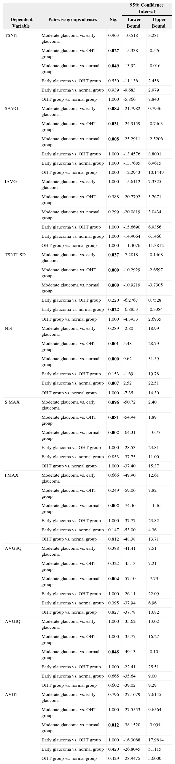
Table 4 reflects the post-hoc range tests (Bonferroni correction) and pairwise multiple comparisons, in order to show the difference between each pair of means at an alpha level of 0.05. Most of the studied parameters decreased significantly in glaucoma patients, compared with the thickness obtained for normal and OHT subjects in the corresponding segments, specially for the moderate glaucoma group. Some of them (SAVG, TSNIT SD for GDx and SMAX for OCT) showed significant differences between moderate and early glaucoma patients.
Bonferroni post hoc range tests and pairwise multiple comparisons showing the difference between each pair of means. Significant differences at the 0.05 level are highlighted (bold)
| 95% Confidence Interval | ||||
| Dependent Variable | Pairwise groups of cases | Sig. | Lower Bound | Upper Bound |
| TSNIT | Moderate glaucoma vs. early glaucoma | 0.963 | -10.518 | 3.281 |
| Moderate glaucoma vs. OHT group | 0.027 | -15.338 | -0.576 | |
| Moderate glaucoma vs. normal group | 0.049 | -13.924 | -0.016 | |
| Early glaucoma vs. OHT group | 0.530 | -11.136 | 2.458 | |
| Early glaucoma vs. normal group | 0.939 | -9.683 | 2.979 | |
| OHT group vs. normal group | 1.000 | -5.866 | 7.840 | |
| SAVG | Moderate glaucoma vs. early glaucoma | 0.084 | -21.7982 | 0.7936 |
| Moderate glaucoma vs. OHT group | 0.031 | -24.9159 | -0.7463 | |
| Moderate glaucoma vs. normal group | 0.008 | -25.2911 | -2.5206 | |
| Early glaucoma vs. OHT group | 1.000 | -13.4576 | 8.8001 | |
| Early glaucoma vs. normal group | 1.000 | -13.7685 | 6.9615 | |
| OHT group vs. normal group | 1.000 | -12.2943 | 10.1449 | |
| IAVG | Moderate glaucoma vs. early glaucoma | 1.000 | -15.6112 | 7.3325 |
| Moderate glaucoma vs. OHT group | 0.388 | -20.7792 | 3.7671 | |
| Moderate glaucoma vs. normal group | 0.299 | -20.0819 | 3.0434 | |
| Early glaucoma vs. OHT group | 1.000 | -15.6690 | 6.9356 | |
| Early glaucoma vs. normal group | 1.000 | -14.9064 | 6.1466 | |
| OHT group vs. normal group | 1.000 | -11.4076 | 11.3812 | |
| TSNIT SD | Moderate glaucoma vs. early glaucoma | 0.037 | -7.2818 | -0.1468 |
| Moderate glaucoma vs. OHT group | 0.000 | -10.2929 | -2.6597 | |
| Moderate glaucoma vs. normal group | 0.000 | -10.9219 | -3.7305 | |
| Early glaucoma vs. OHT group | 0.220 | -6.2767 | 0.7528 | |
| Early glaucoma vs. normal group | 0.022 | -6.8853 | -0.3384 | |
| OHT group vs. normal group | 1.000 | -4.3933 | 2.6935 | |
| NFI | Moderate glaucoma vs. early glaucoma | 0.289 | -2.80 | 18.99 |
| Moderate glaucoma vs. OHT group | 0.001 | 5.48 | 28.79 | |
| Moderate glaucoma vs. normal group | 0.000 | 9.62 | 31.59 | |
| Early glaucoma vs. OHT group | 0.153 | -1.69 | 19.78 | |
| Early glaucoma vs. normal group | 0.007 | 2.52 | 22.51 | |
| OHT group vs. normal group | 1.000 | -7.35 | 14.30 | |
| S MAX | Moderate glaucoma vs. early glaucoma | 0.096 | -50.72 | 2.40 |
| Moderate glaucoma vs. OHT group | 0.081 | -54.94 | 1.89 | |
| Moderate glaucoma vs. normal group | 0.002 | -64.31 | -10.77 | |
| Early glaucoma vs. OHT group | 1.000 | -28.53 | 23.81 | |
| Early glaucoma vs. normal group | 0.853 | -37.75 | 11.00 | |
| OHT group vs. normal group | 1.000 | -37.40 | 15.37 | |
| I MAX | Moderate glaucoma vs. early glaucoma | 0.666 | -49.90 | 12.61 |
| Moderate glaucoma vs. OHT group | 0.249 | -59.06 | 7.82 | |
| Moderate glaucoma vs. normal group | 0.002 | -74.46 | -11.46 | |
| Early glaucoma vs. OHT group | 1.000 | -37.77 | 23.82 | |
| Early glaucoma vs. normal group | 0.147 | -53.00 | 4.36 | |
| OHT group vs. normal group | 0.812 | -48.38 | 13.71 | |
| AVGSQ | Moderate glaucoma vs. early glaucoma | 0.388 | -41.41 | 7.51 |
| Moderate glaucoma vs. OHT group | 0.322 | -45.13 | 7.21 | |
| Moderate glaucoma vs. normal group | 0.004 | -57.10 | -7.79 | |
| Early glaucoma vs. OHT group | 1.000 | -26.11 | 22.09 | |
| Early glaucoma vs. normal group | 0.395 | -37.94 | 6.96 | |
| OHT group vs. normal group | 0.827 | -37.78 | 10.82 | |
| AVGIQ | Moderate glaucoma vs. early glaucoma | 1.000 | -35.62 | 13.02 |
| Moderate glaucoma vs. OHT group | 1.000 | -35.77 | 16.27 | |
| Moderate glaucoma vs. normal group | 0.048 | -49.13 | -0.10 | |
| Early glaucoma vs. OHT group | 1.000 | -22.41 | 25.51 | |
| Early glaucoma vs. normal group | 0.665 | -35.64 | 9.00 | |
| OHT group vs. normal group | 0.602 | -39.02 | 9.29 | |
| AVGT | Moderate glaucoma vs. early glaucoma | 0.796 | -27.1679 | 7.6145 |
| Moderate glaucoma vs. OHT group | 1.000 | -27.5553 | 9.6564 | |
| Moderate glaucoma vs. normal group | 0.012 | -38.1520 | -3.0944 | |
| Early glaucoma vs. OHT group | 1.000 | -16.3068 | 17.9614 | |
| Early glaucoma vs. normal group | 0.420 | -26.8045 | 5.1115 | |
| OHT group vs. normal group | 0.429 | -28.9475 | 5.6000 | |
TSNIT = the calculation circle average thickness; SAVG = the superior 120° average thickness; IAVG = the inferior 120° average thickness; TSNIT SD = the calculation circle standard deviation; NFI = the nerve fiber indicator; SMAX = the maximum thickness in the superior quadrant; IMAX = the maximum thickness in the inferior quadrant; AVGSQ = the average thickness in the superior quadrant; AVGIQ = the average thickness in the inferior quadrant; AVGT = the average thickness for the total circumference.
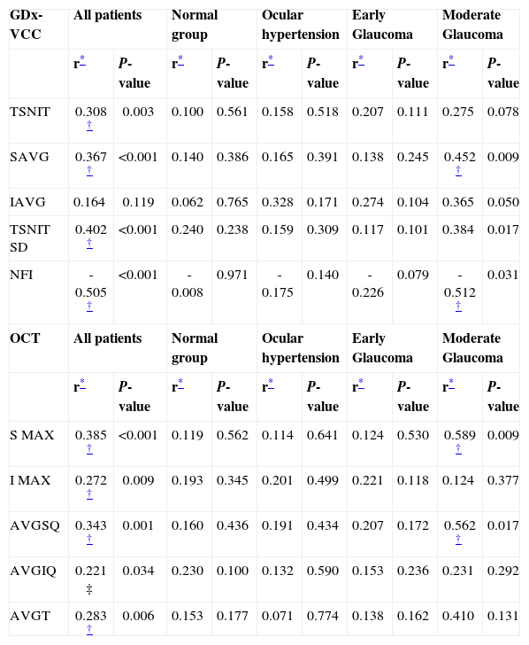
Table 5 illustrates the correlation between RNFL parameters and AAP-MD values. In the entire cohort analysis, significant correlations were observed between TSNIT, SAVG, TSNIT SD, NFI, and all the OCT-generated RNFL thickness. The NFI for the SLP and the SMAX measured with OCT showed the highest correlation value. In the moderate glaucoma group, the SAVG and NFI for the GDx-VCC, and the S MAX and the AVGSQ for OCT showed the highest correlations with MD. These significant correlations were not found in the subgroup analysis of normal, OHT, and early glaucomatous eyes. We believe that these groups showed not significant correlations because in the case of moderate glaucoma patients, the more visual field is lost, the more the RNFL thickness decreases, and also because the regression coefficients are highly influenced by the sample size.
Correlations Between RNFL Analyser Parameters and Mean Deviation, both among all patients and within each of the four groups
| GDx-VCC | All patients | Normal group | Ocular hypertension | Early Glaucoma | Moderate Glaucoma | |||||
| r* | P-value | r* | P-value | r* | P-value | r* | P-value | r* | P-value | |
| TSNIT | 0.308 † | 0.003 | 0.100 | 0.561 | 0.158 | 0.518 | 0.207 | 0.111 | 0.275 | 0.078 |
| SAVG | 0.367 † | <0.001 | 0.140 | 0.386 | 0.165 | 0.391 | 0.138 | 0.245 | 0.452 † | 0.009 |
| IAVG | 0.164 | 0.119 | 0.062 | 0.765 | 0.328 | 0.171 | 0.274 | 0.104 | 0.365 | 0.050 |
| TSNIT SD | 0.402 † | <0.001 | 0.240 | 0.238 | 0.159 | 0.309 | 0.117 | 0.101 | 0.384 | 0.017 |
| NFI | -0.505 † | <0.001 | -0.008 | 0.971 | -0.175 | 0.140 | -0.226 | 0.079 | -0.512 † | 0.031 |
| OCT | All patients | Normal group | Ocular hypertension | Early Glaucoma | Moderate Glaucoma | |||||
| r* | P-value | r* | P-value | r* | P-value | r* | P-value | r* | P-value | |
| S MAX | 0.385 † | <0.001 | 0.119 | 0.562 | 0.114 | 0.641 | 0.124 | 0.530 | 0.589 † | 0.009 |
| I MAX | 0.272 † | 0.009 | 0.193 | 0.345 | 0.201 | 0.499 | 0.221 | 0.118 | 0.124 | 0.377 |
| AVGSQ | 0.343 † | 0.001 | 0.160 | 0.436 | 0.191 | 0.434 | 0.207 | 0.172 | 0.562 † | 0.017 |
| AVGIQ | 0.221 ‡ | 0.034 | 0.230 | 0.100 | 0.132 | 0.590 | 0.153 | 0.236 | 0.231 | 0.292 |
| AVGT | 0.283 † | 0.006 | 0.153 | 0.177 | 0.071 | 0.774 | 0.138 | 0.162 | 0.410 | 0.131 |
GDx-VCC = scanning laser polarimetry; OCT = optical coherence tomography
Significant at 0.05 level (2-tailed); TSNIT = the calculation circle average thickness; SAVG = the superior 120° average thickness; IAVG = the inferior 120° average thickness; TSNIT SD = the calculation circle standard deviation; NFI = the nerve fiber indicator; SMAX = the maximum thickness in the superior quadrant; IMAX = the maximum thickness in the inferior quadrant; AVGSQ = the average thickness in the superior quadrant; AVGIQ = the average thickness in the inferior quadrant; AVGT = the average thickness for the total circumference.
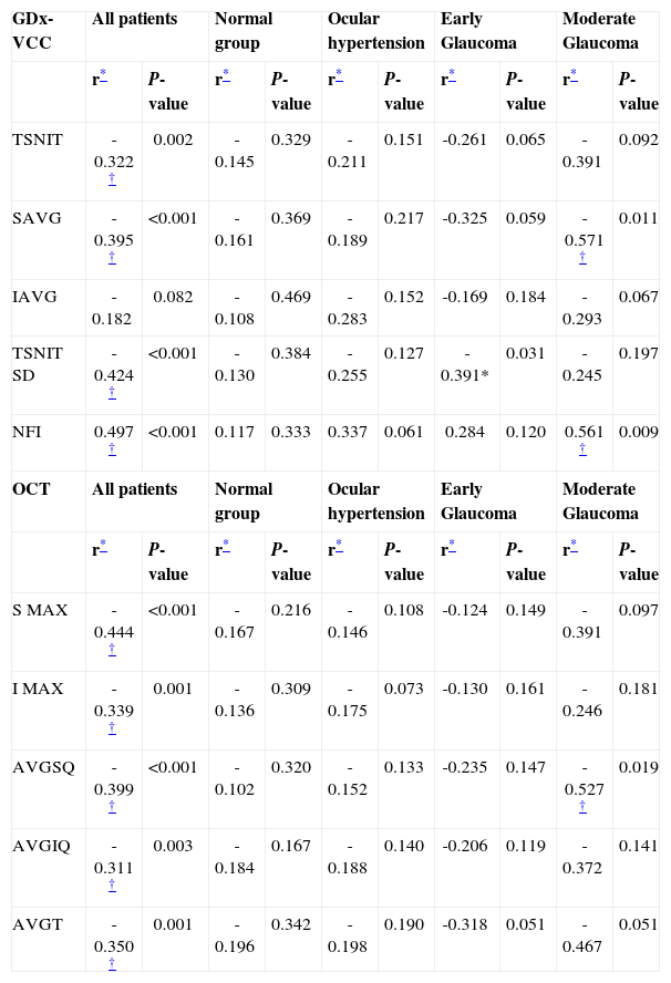
Table 6 shows the correlation between both nerve fiber analyser parameters and visual field PSD. In the entire cohort analysis, significant correlations were observed between TSNIT, SAVG, TSNIT SD, NFI, and all the OCT-generated RNFL thickness. The NFI for the SLP (r=0.497) and the SMAX measured with OCT (r=-0.444) showed the strongest correlation. In the early glaucoma group, the TSNIT SD for GDx-VCC (r=-0.391; P=0.031) was the only one significantly correlated with AAP-PSD. In the moderate glaucoma group, the SAVG (r=-0.571; P=0.011) and the NFI (r=0.561; P=0.009) for SLP, and the AVGSQ (r=0.527; P=0.019) for OCT showed a significant correlation with PSD. SLP and OCT parameters did not correlate with PSD in normal and OHT eyes.
Correlations Between RNFL Analyser Parameters and Pattern Standard Deviation, both among all patients and within each of the four groups
| GDx-VCC | All patients | Normal group | Ocular hypertension | Early Glaucoma | Moderate Glaucoma | |||||
| r* | P-value | r* | P-value | r* | P-value | r* | P-value | r* | P-value | |
| TSNIT | -0.322 † | 0.002 | -0.145 | 0.329 | -0.211 | 0.151 | -0.261 | 0.065 | -0.391 | 0.092 |
| SAVG | -0.395 † | <0.001 | -0.161 | 0.369 | -0.189 | 0.217 | -0.325 | 0.059 | -0.571 † | 0.011 |
| IAVG | -0.182 | 0.082 | -0.108 | 0.469 | -0.283 | 0.152 | -0.169 | 0.184 | -0.293 | 0.067 |
| TSNIT SD | -0.424 † | <0.001 | -0.130 | 0.384 | -0.255 | 0.127 | -0.391* | 0.031 | -0.245 | 0.197 |
| NFI | 0.497 † | <0.001 | 0.117 | 0.333 | 0.337 | 0.061 | 0.284 | 0.120 | 0.561 † | 0.009 |
| OCT | All patients | Normal group | Ocular hypertension | Early Glaucoma | Moderate Glaucoma | |||||
| r* | P-value | r* | P-value | r* | P-value | r* | P-value | r* | P-value | |
| S MAX | -0.444 † | <0.001 | -0.167 | 0.216 | -0.146 | 0.108 | -0.124 | 0.149 | -0.391 | 0.097 |
| I MAX | -0.339 † | 0.001 | -0.136 | 0.309 | -0.175 | 0.073 | -0.130 | 0.161 | -0.246 | 0.181 |
| AVGSQ | -0.399 † | <0.001 | -0.102 | 0.320 | -0.152 | 0.133 | -0.235 | 0.147 | -0.527 † | 0.019 |
| AVGIQ | -0.311 † | 0.003 | -0.184 | 0.167 | -0.188 | 0.140 | -0.206 | 0.119 | -0.372 | 0.141 |
| AVGT | -0.350 † | 0.001 | -0.196 | 0.342 | -0.198 | 0.190 | -0.318 | 0.051 | -0.467 | 0.051 |
GDx-VCC = scanning laser polarimetry; OCT = optical coherence tomography
Significant at 0.05 level (2-tailed); TSNIT = the calculation circle average thickness; SAVG = the superior 120° average thickness; IAVG = the inferior 120° average thickness; TSNIT SD = the calculation circle standard deviation; NFI = the nerve fiber indicator; SMAX = the maximum thickness in the superior quadrant; IMAX = the maximum thickness in the inferior quadrant; AVGSQ = the average thickness in the superior quadrant; AVGIQ = the average thickness in the inferior quadrant; AVGT = the average thickness for the total circumference.
Linear regression was performed to estimate the coefficients between the visual field global indices (independent variables) and the statistical parameters generated by NFA and OCT software (dependent variables), using the stepwise method. For the MD, the only predictor in the model was NFI (r2=0.255; P=0.001), and for the PSD, the predictors in the model were NFI and SMAX (r2=0.296; P=0.014).
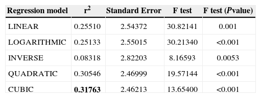
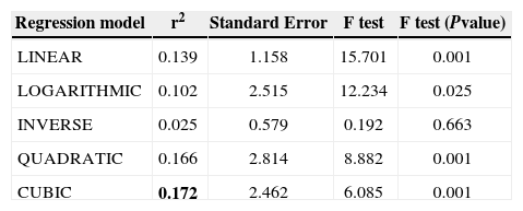
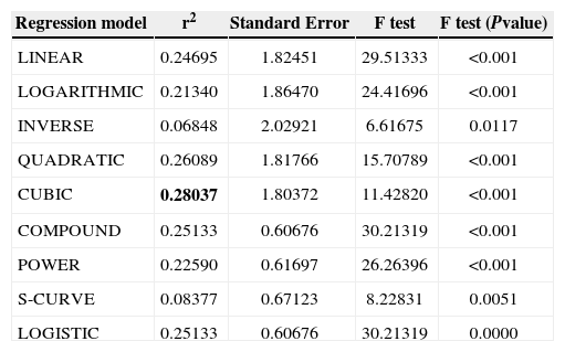
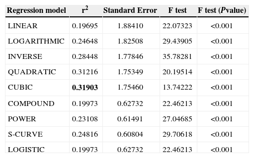
Lastly, curvilinear regression models were used to find out which was the best-fit model. We used VF global indices (MD and PSD) as dependent variables and NFI and SMAX as independent variables since those were the predictors in the linear regression model. As dependent variable MD contains non-positive values, log transform could not be applied and models COMPOUND, POWER, S-CURVE, and LOGISTIC could not be calculated for this dependent variable. Data are shown in tables 7 to 10. The cubic model might be the best to define the relationship between VF indices and SLP/OCT indices because it had the highest coefficient of determination.
Linear and nonlinear regression models for Mean Deviation against the NFI obtained with GDx-VCC. The best-fit model is highlighted (bold)
| Regression model | r2 | Standard Error | F test | F test (Pvalue) |
| LINEAR | 0.25510 | 2.54372 | 30.82141 | 0.001 |
| LOGARITHMIC | 0.25133 | 2.55015 | 30.21340 | <0.001 |
| INVERSE | 0.08318 | 2.82203 | 8.16593 | 0.0053 |
| QUADRATIC | 0.30546 | 2.46999 | 19.57144 | <0.001 |
| CUBIC | 0.31763 | 2.46213 | 13.65400 | <0.001 |
Linear and nonlinear regression models for Mean Deviation against the SMAX obtained with OCT. The best-fit model is highlighted (bold)
| Regression model | r2 | Standard Error | F test | F test (Pvalue) |
| LINEAR | 0.139 | 1.158 | 15.701 | 0.001 |
| LOGARITHMIC | 0.102 | 2.515 | 12.234 | 0.025 |
| INVERSE | 0.025 | 0.579 | 0.192 | 0.663 |
| QUADRATIC | 0.166 | 2.814 | 8.882 | 0.001 |
| CUBIC | 0.172 | 2.462 | 6.085 | 0.001 |
Linear and nonlinear regression models for Pattern Standard Deviation against the NFI obtained with GDx-VCC. The best-fit model is highlighted (bold)
| Regression model | r2 | Standard Error | F test | F test (Pvalue) |
| LINEAR | 0.24695 | 1.82451 | 29.51333 | <0.001 |
| LOGARITHMIC | 0.21340 | 1.86470 | 24.41696 | <0.001 |
| INVERSE | 0.06848 | 2.02921 | 6.61675 | 0.0117 |
| QUADRATIC | 0.26089 | 1.81766 | 15.70789 | <0.001 |
| CUBIC | 0.28037 | 1.80372 | 11.42820 | <0.001 |
| COMPOUND | 0.25133 | 0.60676 | 30.21319 | <0.001 |
| POWER | 0.22590 | 0.61697 | 26.26396 | <0.001 |
| S-CURVE | 0.08377 | 0.67123 | 8.22831 | 0.0051 |
| LOGISTIC | 0.25133 | 0.60676 | 30.21319 | 0.0000 |
Linear and nonlinear regression models for Pattern Standard Deviation against the SMAX obtained with OCT. The best-fit model is highlighted (bold)
| Regression model | r2 | Standard Error | F test | F test (Pvalue) |
| LINEAR | 0.19695 | 1.88410 | 22.07323 | <0.001 |
| LOGARITHMIC | 0.24648 | 1.82508 | 29.43905 | <0.001 |
| INVERSE | 0.28448 | 1.77846 | 35.78281 | <0.001 |
| QUADRATIC | 0.31216 | 1.75349 | 20.19514 | <0.001 |
| CUBIC | 0.31903 | 1.75460 | 13.74222 | <0.001 |
| COMPOUND | 0.19973 | 0.62732 | 22.46213 | <0.001 |
| POWER | 0.23108 | 0.61491 | 27.04685 | <0.001 |
| S-CURVE | 0.24816 | 0.60804 | 29.70618 | <0.001 |
| LOGISTIC | 0.19973 | 0.62732 | 22.46213 | <0.001 |
Assessing the amount of glaucomatous damage is the first step toward the correct management of glaucoma. The damage is usually estimated by observation of structures affected by glaucoma (RNFL and optic disc) and by testing visual function by means of perimetry. It is of great importance to know how the damage to specific structures affects visual function.27
Selective measures of RNFL thickness using these imaging technologies may be able to detect glaucoma before visual field loss occurs: since diffuse RNFL and retinal ganglion cell loss is present in eyes with localized visual field abnormalities;28 it has been reported that RNFL thickness decreased substantially in patients with glaucoma, compared with age-matched healthy subjects.29,30
The purpose of this investigation was to compare these technologies for a cohort of normal, OHT, and glaucomatous subjects. We found that all RNFL measures with Stratus-OCT as well as the TSNIT, SAVG, TSNIT SD and NFI measured with SLP were correlated with visual function global indices, when the entire cohort was analysed.
Different studies have compared newer clinical instruments that measure the structural and functional characteristics of the optic nerve, to the current conventional testing parameters, especially visual field loss. Different nerve fiber analysers correlated strongly with visual field loss, especially among glaucomatous eyes.31,32 This has been proved by means of the Heidelberg Retina Tomograph,29,33,34 confocal scanning laser ophthalmoscopy,35 confocal SLP,36-38 OCT3,39 and stereophotogrammetric measurements of the RNFL at the disc margin.1
Moreover, a high level of correlation between OCTgenerated RNFL thickness, SLP retardation parameters, and visual function has been reported by different authors.6,40,41 However, the correlation between visual field indices and RNFL loss depends on the type of RNFL defect.42 The direct comparison of SLP and OCT results with visual field indices was the main purpose of our investigation.
Correlations Between GDx-VCC and AAPSLP makes use of the birefringence features of ganglion cell axons, measuring the linear retardation in order to calculate RNFL thickness. Recently, GDx was modified into the GDx- VCC, which includes a variable cornea compensator (VCC) that uses macular-based strategies for neutralization of corneal polarization magnitude. It has been stated that, compared with fixed compensation, VCC improves the relationship between mean-based SLP retardation parameters and visual function, particularly with standard automated perimetry visual field MD and PSD.7,43,44,(Garcia-Sánchez J, et al. IOVS 1998;39(Suppl): S933.Abstract 4298) Moreover, the nerve fiber indicator was the best parameter from the GDx-VCC to discriminate between healthy eyes and eyes with glaucomatous visual field loss using the receiver operating characteristic curves (AUC=0.91).30
In this study, we found that GDX-VCC mean-based retardation parameters were correlated with AAP MD and PSD as outcome variables. These findings are consistent with the results reported by other authors. It has been shown36 that RNFL thickness decreases are associated with an increase of field defects (MD value) both globally and by hemi-field/hemiretina. It has also been found8 that there is a weaker correlation between mean-based retardation parameters and visual function (r2=0.17 to 0.27), as compared with constructed retardation parameters (modulation parameters, ratio parameters, and neural network number; r2=0.36 to 0.51) using SLP with fixed compensation. Some authors,31,43 (Garcia-Sánchez J, et al. IOVS 1998;39(Suppl): S933.Abstract 4298) have reported that constructed SLP parameters (modulation, ratio, neural network number, and linear discriminant function values) have greater discriminating power compared with mean-based parameters. In fact, in this study, a GDx-VCC constructed parameter, the NFI, showed the strongest correlation between the SLP parameters and the VF global indices (tables 4 and 5), which suggests that GDx-VCC could be a well suited technique for the early detection of glaucoma.
Although previous studies have demonstrated similar discriminating power for the detection of early to moderate glaucoma,6,40,43 mean-based retardation parameters obtained with SLP (integral and average thickness values) have been reported to have a relatively weak correlation with RNFL thickness yielded by OCT.8 However, in this study, we found a better correlation in the presence of a significant visual field defect (moderate glaucoma group) and a worse correlation when the visual field was close to normal (early glaucoma patients), which is in agreement with other authors’45 findings. Unfortunately, the moderate glaucoma group is a population segment that presents to clinicians fewer diagnostic complications than early glaucoma patients, since a significant visual field loss is easy to detect by perimetry alone. The worse correlation between early glaucoma patients compared to moderate glaucoma patients could it be due to the so-called functional reserve. On the other hand, it has been stated that the lack of correlation between VF and RNFL parameters in early glaucoma patients could be due to the moderate discriminating power of the commercially available instruments, combined with the great inter-individual variability in RNFL thickness, which causes a significant overlap between normal, OHT and early glaucoma patients.27 Moreover, histological studies showed that 25% to 40% of retinal ganglion cells axons are lost before abnormality changes are detected through automated VF testing,46 probably because of the logarithmic scale used in VF.
In addition, the only significant correlation for the early glaucoma group between the GDx-VCC parameters and VF global indices was between TSNIT SD and AAP PSD. We believe that TSNIT SD could be the best GDx-VCC parameter to differentiate early cases of glaucoma (Table 5).
Correlations Between Stratus-OCT and AAPOCT is based on the measurement of the reflectance of the posterior segment structures and incorporates a mathematical algorithm capable of localizing the anterior and the posterior limits of the RNFL. It has proved to be useful as a glaucoma-screening tool in the general population,39 because RNFL measurements by OCT have revealed NFL thinning in areas corresponding to visual field defects.47 Moreover, regional OCT, which measured RNFL thinning in glaucoma patients, was reported to be associated with decreases in VF zone sensitivity,22 and it was stated48 that OCT is a promising tool to provide quantitative data about the location and the extent of retinal nerve fiber layer injury in glaucoma.
In this investigation, OCT provided the strongest correlation between RNFL thickness and MD or PSD for the entire cohort group (Tables 5 and 6), because the mean Pearson's correlation coefficient for OCT was significantly higher than for GDx-VCC. These results agree with those obtained by other authors3,11 and the higher association with visual function in Stratus-OCT RNFL measurements, compared with that carried out with GDx-VCC, suggest that optical coherence tomography might be a better approach to the evaluation of structure/function relationships. Moreover, OCT could attain a higher resolution than GDx
In the current study, the resulting correlation values between mean global RNFL thickness on OCT and each of the two AAP ratios were similar and did not exhibit large differences (PSD=-0.3686; MD=0.3008). Others studies had reported contradictory results. El Beltagi et al.22 reported that localized RNFL thinning, measured by OCT, is topographically related to decreased localized AAP sensitivity in glaucoma patients.
On the other hand, Hoh et al.8 showed a stronger correlation between RNFL measurements with AAP MD rather than with AAP corrected PSD. This finding suggests a week relationship between structural and functional measurements in glaucoma and, therefore, the results of these ancillary tests should be interpreted jointly to increase diagnostic accuracy.26
Regression ModelsIn the present study, dependent and independent variables were quantitative, and categorization of paired (X,Y) data is generally not quite linear. They are generally more S-shaped, though very shallow curves can be almost linear. There are already several publications11,44,49 indicating the lack of a linear relationship between functional and structural losses. The top candidates are cubic smoothing spline and logistic functions, because they have this particular shape. Garway- Heath et al.49 demonstrated, in a group of 74 healthy and glaucomatous eyes, that there was significant linear and quadratic relationships between temporal neuroretinal rim area (in square millimeters) measured with retinal tomography, and visual sensitivity (dB) measured by means of standard automated perimetry. Coefficient of determination (r2) for the linear fit was 0.30 and r2 for the quadratic fit was 0.38. Schlottmann et al.44 showed small but significant improvements in structure–function associations with logarithmic regression using analysis of model residuals. Leung et al.11 used linear and four nonlinear models to assess the association between global visual sensitivity and mean RNFL thickness in healthy, suspect, and glaucomatous eyes, as measured with the Stratus OCT and GDx VCC, and found secondand third-order polynomial curves, respectively, to be better fits than lines when visual sensitivity was expressed in decibels. In the present study, linear regression models showed that the independent variable MD was correlated with the dependent variable NFI and the independent variable PSD was correlated with the dependent variables NFI and SMAX. After that, we calculated the curvilinear regression models adjusting the model to the data points and, according to our results, the cubic curve estimation turned out to be the best fit (in terms of r2), as well as the best theoretical match to the expected shape of our data, when compared to the various offered curves. Anyway, the differences of the determination coefficients were very small, so it cannot really be stated that the cubic model is much better than the linear one.
RNFL Measurements in Glaucomatous, OHT and Normal EyesThe results from this study show that, with the use of both technologies, significant structural differences can be observed between moderate glaucoma patients and nonglaucomatous eyes. Moreover, some parameters in glaucomatous eyes showed significant differences compared with normal eyes (Tables 5 and 6). Furthermore, the magnitude of RNFL thinning is related to the decrease of AAP sensitivity. These findings provide validity for both nerve fiber analysers as diagnostic tools, because the results agree with previous knowledge regarding tissue morphology in glaucoma.
As was previously exposed, most parameters in early and moderate glaucomatous eyes showed significant differences with normal eyes. However, there were few significant differences between normal and OHT eyes in terms of the parameters under consideration in this study. Although mean RNFL thickness (Stratus-OCT) and ellipse average (GDx-VCC) measurements were smaller in OHT than in normal eyes, these differences were not statistically significant. These two groups exhibited similar results because, from the functional and anatomic point of view, they have similar characteristics. Our results were in agreement with previous reports3,8,16,35 and disagree with others that found structural differences between these groups11,50 or even between healthy eyes and eyes with localized RNFL defects without VF loss (preperimetric glaucoma).51
It should be noted that it is difficult to compare associations between structure and function across studies because the strength of the correlation coefficient is dependent on many features of the study design. The diagnostic groups included, the severity of the disease for the glaucoma patients, and the range of the measurements will have an impact on the resulting correlation values. For example, weak correlations between RNFL measures and visual field MD and PSD would be expected in studies of healthy subjects and OHT patients without visual field loss, because the visual field indices would all have a limited range. Also, the sample size could probably play a role when the correlations between RNFL thickness and VF sensitivity are determined.
In conclusion, quantitative measurements of RNFL thickness using both GDx-VCC and Stratus-OCT correlated moderately with VF indices for moderate glaucoma patients. In a few cases early glaucomatous eyes showed only borderline correlations and in most cases were not correlated with neither MD or PSD. Cross-sectional studies have limitations when examining the relationship between structural parameters and function because they can assist in determining which parameters are associated to the visual function but they cannot address the temporal relationship between structure and function. Therefore, longitudinal studies must be carried out in order to obtain information regarding how the visual field reflects the anatomic damages that occur in the course of the glaucomatous disease.
Optic-nerve imaging technologies continue to improve, both in terms of their technological ability to measure, and in terms of software to evaluate the optic nerve. These SLP and OCT versions had similar performance to separate glaucomatous and non-glaucomatous populations, but they were unable to differentiate normal from OHT populations in this cohort (Tables 5 and 6). A constructed retardation parameter, the NFI, was the one that was able to discriminate best between different stages of glaucoma in the present study. But, at the moment, none of these instruments is sufficient in and of itself to replace the traditional methods of examination. Either imaging technologies or visual field assessment may show the first evidence of glaucomatous damage; therefore, the combination of optic nerve head parameters and visual field results could improve glaucoma diagnosis and follow-up52. Physician judgment remains crucial in evaluating the output of these devices and in incorporating that into the diagnosis and management of individual patients. Future improvement in imaging technology, which provides higher resolution and better reproducibility, may enhance their sensitivity and specificity, increasing their usefulness for population screening.
Sources of support: Supported by a grant from the University of Valencia (UV-3691).


