


To describe the individual virtual eye, a computer model of a human eye with respect to its optical properties. It is based on measurements of an individual person and one of its major application is calculating intraocular lenses (IOLs) for cataract surgery.
MethodsThe model is constructed from an eye's geometry, including axial length and topographic measurements of the anterior corneal surface. All optical components of a pseudophakic eye are modeled with computer scientific methods. A spline-based interpolation method efficiently includes data from corneal topographic measurements. The geometrical optical properties, such as the wavefront aberration, are simulated with real ray-tracing using Snell's law. Optical components can be calculated using computer scientific optimization procedures. The geometry of customized aspheric IOLs was calculated for 32 eyes and the resulting wavefront aberration was investigated.
ResultsThe more complex the calculated IOL is, the lower the residual wavefront error is. Spherical IOLs are only able to correct for the defocus, while toric IOLs also eliminate astigmatism. Spherical aberration is additionally reduced by aspheric and toric aspheric IOLs. The efficient implementation of time-critical numerical ray-tracing and optimization procedures allows for short calculation times, which may lead to a practicable method integrated in some device.
ConclusionsThe individual virtual eye allows for simulations and calculations regarding geometrical optics for individual persons. This leads to clinical applications like IOL calculation, with the potential to overcome the limitations of those current calculation methods that are based on paraxial optics, exemplary shown by calculating customized aspheric IOLs.
Describir el ojo virtual individualizado, que es un modelo computacional de ojo humano con respecto a sus propiedades ópticas. Está basado en las medidas realizadas en cada persona, de manera individual. Una de sus principales aplicaciones es el cálculo de lentes intraoculares (LIO) para cirugía de cataratas.
MétodosEl modelo está construido a partir de datos de geometría ocular; en particular, la longitud axial y las medidas topográficas de la cara anterior de la córnea. Todos los componentes ópticos de un ojo pseudofáquico se modelan por medio de métodos computacionales científicos. El método de interpolación por splines permite incluir de manera eficiente los datos obtenidos en las medidas de topografía corneal. Las propiedades relacionadas con la óptica geométrica, como el patrón de aberración del frente de onda, se obtienen a partir de la simulación de un trazado de rayos reales, el cual emplea la ley de Snell. Los componentes ópticos se pueden calcular empleando procedimientos computacionales de optimización. Para 32 ojos distintos, se calculó la geometría de la correspondiente LIO asférica personalizada y se analizó la aberración del frente de onda resultante.
ResultadosCuanto más compleja es la LIO calculada, menor resulta ser el error residual del frente de onda. Las LIO esféricas sólo son capaces de corregir el desenfoque, mientras que las LIO tóricas también permiten eliminar el astigmatismo. De manera adicional, también disminuye la aberración esférica cuando se emplean LIO asféricas y LIO asféricas tóricas. La implementación eficiente de aquellos procedimientos numéricos potencialmente lentos de trazado de rayos y de optimización permite lograr unos tiempos de cálculo reducidos. Esto puede permitir desarrollar métodos que se podrían integrar en un dispositivo de medida.
ConclusionesEl ojo virtual individualizado permite realizar simulaciones y cálculos relativos a las propiedades de óptica geométrica de sujetos individuales. Esto puede posibilitar el desarrollo de aplicaciones clínicas, tales como el cálculo de LIO, que podrían en principio superar las limitaciones impuestas por aquellos métodos de cálculo actuales basados en la óptica paraxial. Un ejemplo aquí descrito es el cálculo de LIO asféricas personalizadas.
Geometric optics or ray optics assumes that the wavelength of the light is sufficiently small so that the light propagation can be described in terms of rays. The path of the rays is determined by reflection and refraction. The latter is defined by Snell's law of refraction. A ray, obeying Snell's law, is called exact ray or real ray. Analyzing optical systems by tracing many rays based on Snell's law is therefore known as exact-ray tracing, finite-ray tracing or real ray-tracing (RRT), a common approach in technical optics.1,2
Such a real ray is opposed to a paraxial ray obeying the paraxial approximation of Snell's law. This first-order approximation of Snell's law is a simplification of geometric optics, in that it assumes small angles of the rays with respect to one common optical axis. Every point in the object space can be one-to-one transformed into a point in the image space. Paraxial optics provides a quick overview about the optical properties of an optical system; however, it is no more than an idealized model.3 Moreover, lens optics is based on paraxial optics, where the essential quantity describing optical components is the diopter. In contrast, analysing optical systems with RRT leads to a more comprehensive description, especially including effects of irregular surface shapes. In terms of geometrical optics, every deviation from a perfect optical system can be quantified in terms of the so called optical aberrations.
The application of RRT in ophthalmology in general is not new. It has been used to address various issues, typically as soon as paraxial optics is not sufficient to describe optical properties accurately. One field of application is corneal refractive surgery, where the shape of the cornea is modified by means of some surgical procedure, for example by removing a certain amount of tissue—the so called ablation profile—with an excimer laser.
Klonos et al. did some early investigations of ablation profiles in a model eye.4 Ortiz et al. used RRT for choosing the optimal ablation parameters from individualized eye models.5-7 Most studies using RRT in the context of simulating and analyzing ablation profiles for refractive surgery are mainly focused on corneal wavefront aberration and they all include measured anterior corneal surface data, the so called corneal topography.8-16
Intraocular lenses (IOLs) are a second major field of investigation for RRT. IOLs are the artificial lenses that are used in cataract surgery to replace the cloudy human crystalline lens. There is literature that evaluates IOL designs (mainly spherical versus aspheric) with RRT, without making use of corneal topography data,17-23 while others explicitly use measured corneal topographies;24-29 some studies additionally included polychromatic effects.20,28 Franchini et al. used real ray- tracing to study different lens-edge designs by analyzing the reflected glare images.30 Ho et al. investigated accommodating IOLs using RRT.31 There is also some literature regarding the actual calculation—beyond a simple analysis—of optical components, such as IOLs, employing RRT.32-40
There are other published studies that are not directly IOL- or refractive-surgery-related; for instance, some studies used RRT for the analysis of schematic eyes.41-43 Fink et al. simulated human optics with real ray- tracing.44-46 Others carried out investigations using RRT based on measured corneal topography data.47-50 Sarver et al. also used corneal topography data and are principally capable of calculating optical components with their Visual Optics Lab* program.51 Only few authors did RRT calculations including a gradient-index model of the human crystalline lens.4,52-56
The individual virtual eye is a computer model of a human eye that accounts for its optical properties, and which is designed to contribute to all fields of research where ray tracing has been used so far. However, it does not include yet the human crystalline lens. Established schematic eye models, such as Gullstrand's model,57 are intended to represent properties of an average eye based on averaged population measurements. In contrast, the individual virtual eye is based on measurements of a single person. The geometry of the eye is important, including axial length and anterior corneal surface. While theoretical surfaces can also be used, the focus lies on the inclusion of measured corneal topography data.
All optical components of a pseudophakic eye –an eye with an artificial lens– are modeled by means of computer methods. Based on this virtual eye model, its geometrical optics properties, such as the wavefront aberration, can be simulated with RRT. Moreover, optical components can be calculated using computer optimization procedures; which leads to potential clinical application fields in ophthalmology. Most studies using ray tracing found in literature investigate specific issues in vision science and often rely on commercially available optical design programs like ASAP (Breault Research Organization, Inc., Tucson, AZ), CODE V (Optical Research Associates, Pasadena, CA), OSLO (Lambda Research Corporation, Littleton, MA), or ZEMAX (ZEMAX Development Corporation, Bellevue, WA). In contrast, this study focuses on the development of an autonomous computer eye model that may serve as basis for various applications in the clinical practice. The virtual eye is designed and implemented in a way that would allow for its integration in a single medical device, thus gaining in efficiency and usability.
A first application of the individual virtual eye was the calculation of spherical IOLs as described in a previous work.58 In the present paper, the individual virtual eye and the RRT calculation methods are described in more detail, especially regarding the computer technical implementation. Based on measured patient data customized aspheric lenses are calculated, thus showing the capability of the method to deal with advanced lens geometry.
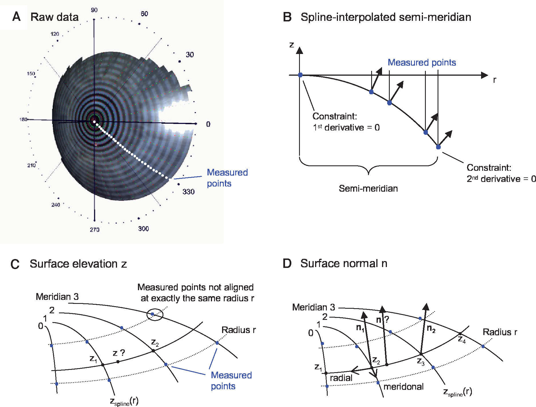
MethodsOptical Components of the Virtual EyeThe anterior cornea is the most dominant refracting surface of the human eye and is constructed from videotopography data. Common to most topography systems using Placido rings is the analysis of the ring positions from the center of the topography along its meridians. The raw corneal elevation data is typically given as values at a set of discrete measurement positions aligned along meridians, as shown in figure 1A. For the ray-tracing procedure, there has to be the possibility to determine the surface elevation and the surface normal at any generic position, not only at the discrete measured positions. Therefore, the following interpolation schema is used:

Spline-based interpolation method for corneal topography data to obtain surface elevation data and normals at any generic position. A. The points for which raw elevation readings are provided by a topography device are distributed at discrete positions along meridians. B. A functional cubic spline interpolation is done for each semi-meridian. By using these functional representations of the semi-meridians, the C. Surface elevation and D. Surface normals are calculated.
Figure 1B shows one semi-meridian consisting of measured points. At r = 0 the vertex point is added. Without loss of generality, only two rings are shown. A functional cubic spline interpolation is performed for each individual semimeridian. Two constraints are set: at the vertex point the first derivative of the spline function has to be zero and at the last ring's edge the second derivative is set to zero. As a result of the first constraint the surface normal at the vertex always coincides with the z-axis. This spline interpolation leads to a function zspline(r) and to its derivative zspline‘(r), which can be evaluated at a general radii r.
Figure 1C outlines the calculation of an elevation z at any generic position:
- 1.
Calculation of the elevations z1 and z2 via zspline(r) of adjacent meridians with the same radius r (this is important, because the measurement points are usually not aligned along the same radius r this would be only the case when the cornea is exactly rotationally symmetric.)
- 2.
Calculation of the elevation z as a linear interpolation along the circular arc.
Figure 1D outlines the calculation of a surface normal n at any generic position:
- 1.
Calculation of the surface normals n1 and n2:
- a.
Meridonal: via the derivative zspline‘(r) of adjacent meridians
- b.
Radial: via a parabolic interpolation of adjacent elevations
- a.
- 2.
Calculation of the surface normal n as a linear vectorinterpolation of n1 and n2.
The spline interpolation of the semi-meridians is done in a pre-processing step once. No computationally expensive calculations are necessary in time-critical procedures. This is an important issue, since ray-surface intersection calculations dominate the ray-tracing calculations. Another approach could have been to approximate (instead of interpolate) the elevation data, for example with Zernike polynomials. Once fitted, this approach could also provide elevation and normals in a fast and elegant way.
However, one has to ensure that enough Zernike coefficients are used, so that the approximation is exact enough – anyway, this approach remains an approximation. The presented interpolation schema was used to stick as close to the measured values as possible.
The difference in refraction indices at the anterior corneal surface between air and stroma is much bigger than the difference between stroma and aqueous humor at the posterior corneal surface. Talking in terms of paraxial optics, in an average human eye the anterior corneal surface has an approximate refractive power of +48 D, while the posterior one only has -6 D.59
Therefore, the anterior corneal surface is very dominant with respect to the posterior one, even though this surface is not, by any means, negligible. In the virtual eye, it is modeled just as the anterior cornea, by means of the described spline-interpolated schema; when there are no measurements of the surface available, the corresponding data have to be either estimated from the anterior corneal surface or standard values matching the population average have to be used.
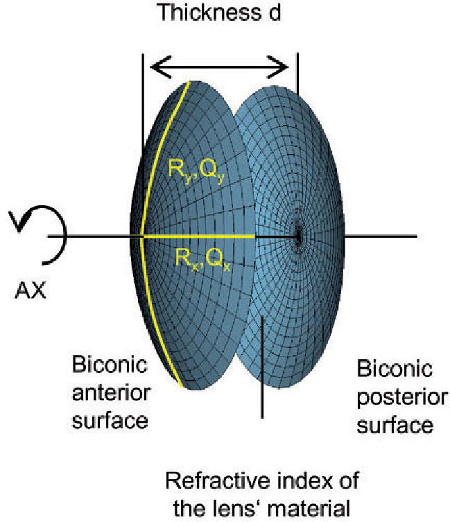
The virtual lens is modeled by theoretical surfaces. To be able to model both toricity and asphericity, a biconic surface is used:52
Rx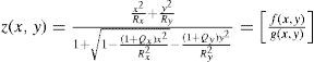
radius of curvature in the x direction
Ryradius of curvature in the y direction
Qxasphericity in the x direction
Qyasphericity in the y direction
Two radii of curvature and two corresponding asphericities are used for specification. Each pair of radius and asphericity describes one conic section; the two conic sections are perpendicular to each other. For Rx = Ry and Qx = 0 and Qy = 0, the formula describes a sphere. For Rx ≠ Ry and Qx = 0 and Qy = 0, the resulting surface is similar (though not identical) to a part of a torus. For Rx = Ry and Qx = Qy and Qy ≠ 0, the formula represents a conicoid.
The axis of a lens does not have to lie exactly on the x or y axis; this is handled by means of a simple variable substitution that is equal to a local coordinate transformation by a rotation matrix. The numerator f(x,y) and denominator g(x,y) of the biconic formula can both be differentiated. Partial derivative with respect to x:
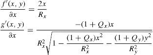
Partial derivative with respect to y:

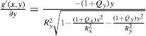
By using the quotient rule
the biconic formula can be easily differentiated using f’(x,y) and g’(x,y). This enables the calculation of the surface normal at any generic position, which is crucial for the raysurface intersection calculations that are required in the ray tracing process.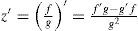
The virtual lens is completely defined by two refracting biconic surfaces, a thickness and the refractive index of the lens’ material (Figure 2). While a standard spherical lens’ geometry is restricted to spherical surfaces, the modeling with a biconic surface allows for various possibilities:
- •
Toric lenses can be modeled by using different radii Rx and Ry.
- •
Aspheric lenses result from using non-zero values for Q.
- •
Design issues can be assessed, like biconvex or planoconvex lens design.

Toric and aspheric surfaces can be used for the anterior surface, the posterior surface, or both. Lenses can be designed to be either symmetric or asymmetric, and so on.
Real Ray-TracingOnce the virtual eye is constructed, consisting of the anterior and posterior corneal surfaces as well as the lens, a RRT procedure can be performed. A light source located in the object space is projected onto the virtual retina. This is done by sending a number of light rays through the virtual eye. In principle, this light source can be located anywhere in object space. However, the most common case is to assume that this light source is located at an infinite distance from the eye; this corresponds to the simulation of distance viewing. In this case, the light rays can be assumed to be a bunch of rays parallel to the axis of the eye and uniformly distributed following a square pattern. These rays firstly reach the anterior cornea. The pupil limits the amount of light entering the eye. The entrance pupil is the image of the real pupil in the object space.59 Its dimensions can be either direct measurements (from a topography system, for example) or theoretical values. All rays falling outside this entrance pupil are neglected.
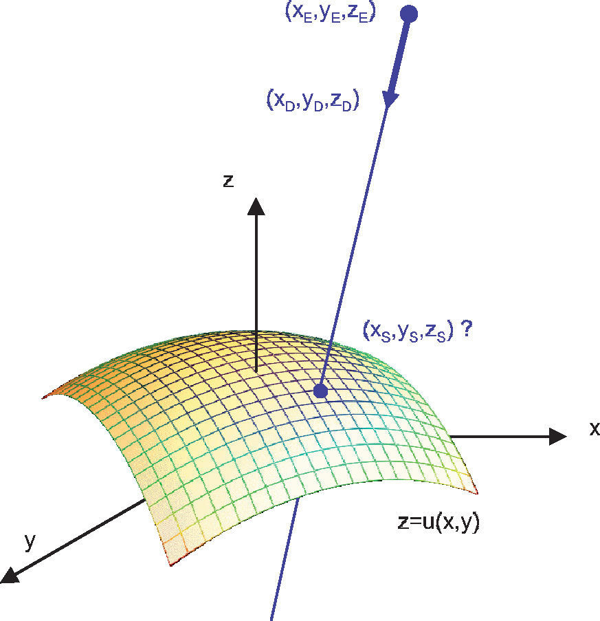
As the light rays travel through the virtual eye, the dominant task is to calculate the intersections between rays and surfaces, as well as the surface normals at those points, thus determining the new direction of the ray according to Snell's law of refraction. All surfaces included in the virtual eye are described by a function u(x,y) (Figure 3). A light ray emerging from a position E and travelling in the direction D can be written in parametric form as a function of t:
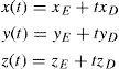

The calculation of the parameter tS that satisfies the following equation results in the intersection:
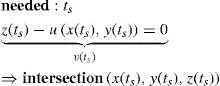
When the surface specified by u is a sphere, the solution of this equation leads to a quadratic equation, and can therefore be calculated algebraically in an efficient way. When u corresponds to the biconic formula, this leads to a 4th degree polynomial. The solution of this polynomial is a large formula and, therefore, a general numeric method was preferred: numeric root-finding via Van Wijngaarden-Dekker-Brent's Method.60 In contrast to other root-finding algorithms, this method does not use a symbolic derivative of the function v, which makes it applicable even when the function u results from a spline-interpolated measured cornea and a derivative of the function is not directly available.
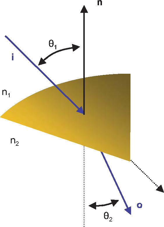
Once the intersection with a surface is determined, the surface normal is calculated. Knowing the direction of the ray before refraction i, the surface normal n and the refractive indices n1 and n2 of the two media that are separated by the surface, the new direction o of the ray after refraction can be calculated (Figure 4) according to Snell's law by using Heckbert's method:61
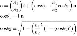

This vectorial form has the advantage that the cosines of the angles do not have to be calculated, making it an elegant way of calculating Snell's law in the three dimensional space. Once the rays traced through the virtual eye have gone through all the refracting surfaces (cornea and lens), they finally reach the virtual retina. While a real retina has some radius of curvature, for the sake of simplicity the virtual retina is assumed to be a plane. The intersections of all rays with this retinal plane make up a spot diagram (Figure 5). In the case of a perfect optical system (in terms of geometrical optics), i.e. free from aberrations, a point in the object space would be projected onto a unique point in the image space (the retina). Therefore all rays emerging from the point light source, then traced through the virtual eye would finally reach the retina at one point of infinitesimally small size. The more the optical system deviates from the ideal state, the bigger the spot size will be. From the two-dimensional spot diagram the root mean square (RMS) spot size can be calculated62 [p. 178 f.]:
n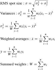
number of rays traced
Wiweighting factor for each ray

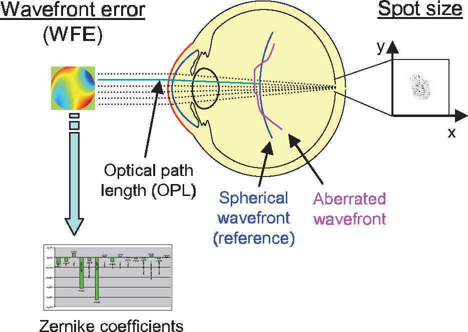
Two criteria to assess optical quality. The spot size is calculated from the spot distribution at the virtual retina. The wavefront aberration is calculated as the difference in optical path length with respect to a reference wavefront. The latter can be approximated with Zernike polynomials for further analysis.
The weights for each ray enable the incorporation of the Stiles-Crawford effect.63 The effect refers to the directional sensitivity of the cone photoreceptors of the human eye, and can be simulated by means of an apodization filter placed at the pupil. Therefore, the rays are weighted depending on their distance to the pupil center, which is a reasonable approximation59 [p. 125]:
r [mm]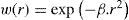
ray distance from pupil center
βStiles-Crawford coefficient
Another metrics often used to quantify the optical quality is the wavefront aberration or the RMS of the wavefront error (WFE). The wavefront aberration is the offset between a spherical reference wavefront and the actual aberrated wavefront (Figure 5). This wavefront aberration can be calculated as follows: first, the intersections of the rays with a sphere representing the reference wavefront are calculated. Then the optical path length (OPL) to these intersections is calculated as the geometric path length multiplied by the refractive index of the corresponding medium. For each ray, we calculate the difference between the actual OPL and the reference OPL. This results in a wavefront aberration function, which can be used to calculate the RMS wavefront error or which can be approximated by Zernike polynomials via least-square fitting. In both cases a weighting of the rays is possible, just as it was in the case where the RMS spot size was used as metrics of optical quality. Zernike polynomials are a set of orthogonal polynomials that provide a very compact description of a potentially complex wavefront shape and that allow for the distinction of different kinds of aberrations.2,62
Optimization ProcedureThe optimization procedure is the key process for the calculation of optical components in the virtual eye. First of all, a function F(v1, v2, …) is constructed, which receives some input variables vi. These are the parameters whose value has to be calculated. Each function evaluation consist of a complete ray-tracing iteration, as described in the preceding section. The output of the function is the optimization criterion, either the RMS spot size or the wavefront error. In an optimization process this function F is minimized, which implies that the aberrations are minimized. As input variables, parameters describing the geometry of the optical component are chosen.
This leads to one or more parameters, depending on the complexity of the component; the optimization procedure is therefore one- or multi-dimensional.
The function F that has to be minimized is nonlinear and no derivative is directly available. In general, the task of finding a global minimum of such a function is very difficult.60 [p. 394] Sophisticated attempts to obtain a solution include methods like genetic algorithms or adaptive simulated annealing and are, for example, implemented for the purpose of optimizing complex optical systems in commercial ray-tracing packages such as OSLO (Lambda Research Corporation, Littleton, MA).62 [p. 220 ff.] Although no formal proof is presented, it turned out that for every calculation performed with the individual virtual eye so far, an algorithm for finding the local minimum of the function F was sufficient. This evidence is the result of an empirical approach: the optimization procedure was initiated at various different starting conditions, but always yielded the same minimum. Therefore, it is very likely that this local minimum was also the global minimum. For the one-dimensional case Brent's method60 [p. 402 ff.] was used. The multi-dimensional minimization is done with Powell's method60 [p. 412 ff.] which, again, uses Brent's method as a sub-algorithm. In all cases no derivative of F is needed.
Calculation of Customized IOLs for PatientsIn the present study, the individual virtual eye was used to calculate advanced IOL geometries, like customized toric and/or aspheric IOLs. The term “customized” means that the IOLs are calculated for an individual patient. After calculating the customized IOLs the remaining wavefront aberration is analyzed with RRT. The results are then analyzed, comparing the performance of the different kinds of IOLs.
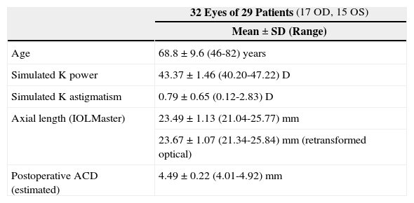
For the calculations and simulations the measurements of 32 eyes of 29 caucasian patients that had undergone cataract surgery without complications at the University Eye Hospital Tübingen were used retrospectively (Table 1). A schematic view of the individual virtual eye and the calculation procedure is shown in figure 6. The anterior corneal surface was measured preoperatively with a CScan (Technomed GmbH, Germany) videotopometer. Axial length was measured with an IOLMaster (Carl Zeiss Meditec AG, Germany) and the readings were then transformed into an optical length value. This is necessary because the IOLMaster is calibrated by the manufacturer against acoustic measurement devices (immersion ultrasound), which measure the length from the cornea to the inner limiting membrane. For ray tracing, the optical length to the retinal pigment epithelium is needed, which is in fact what is internally measured by the IOLMaster using partial coherence interferometry (PCI). Therefore, this value can be retransformed (recovered) from acoustical length readings, according to Olsen et al.64 The posterior corneal surface data were estimated from the anterior surface ones using a constant back-to-front ratio of 0.81.59 [p. 12] Corneal thickness was assumed to be 0.5 mm. The anterior chamber depth (ACD) was estimated from axial length, using regression data based on PCI measurements of the SA60AT lens.65 The refractive indices of Gullstrand's eye model were used.57 [p. 300] In each ray-tracing iteration, a square matrix of 50x50 uniformly distributed rays were traced through the virtual eye. After carrying out the multi-dimensional optimization process as described above (using each patient eye's individual spline-interpolated elevation data, axial length and ACD), the following types of IOLs are calculated (seefigure 7):
- (A)
a spherical IOL (calculation of R =>1-dimensional optimization)
- (B)
an aspheric IOL (calculation of R & Q => 2-dim. optimization)
- (C)
a toric IOL (calculation of R1 & R2 & AX => 3-dim. optimization)
- (D)
a toric aspheric IOL (calculation of R1 & R2 & AX & Q => 4-dim. optimization)
Baseline patient data
| 32 Eyes of 29 Patients (17 OD, 15 OS) | |
| Mean ± SD (Range) | |
| Age | 68.8 ± 9.6 (46-82) years |
| Simulated K power | 43.37 ± 1.46 (40.20-47.22) D |
| Simulated K astigmatism | 0.79 ± 0.65 (0.12-2.83) D |
| Axial length (IOLMaster) | 23.49 ± 1.13 (21.04-25.77) mm |
| 23.67 ± 1.07 (21.34-25.84) mm (retransformed optical) | |
| Postoperative ACD (estimated) | 4.49 ± 0.22 (4.01-4.92) mm |
ACD: anterior chamber depth. K: keratometric data.

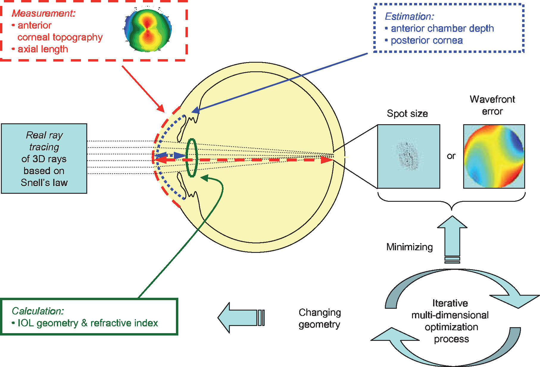
Schematic view of the individual virtual eye. The anterior corneal surface and the axial length are typically measured, while other parameters, such as the posterior cornea and the lens position, are estimated. Optical components are calculated by means of an optimization procedure that minimizes either the wavefront error or the spot size. Therefore, many iterations of the ray-tracing procedure are necessary.

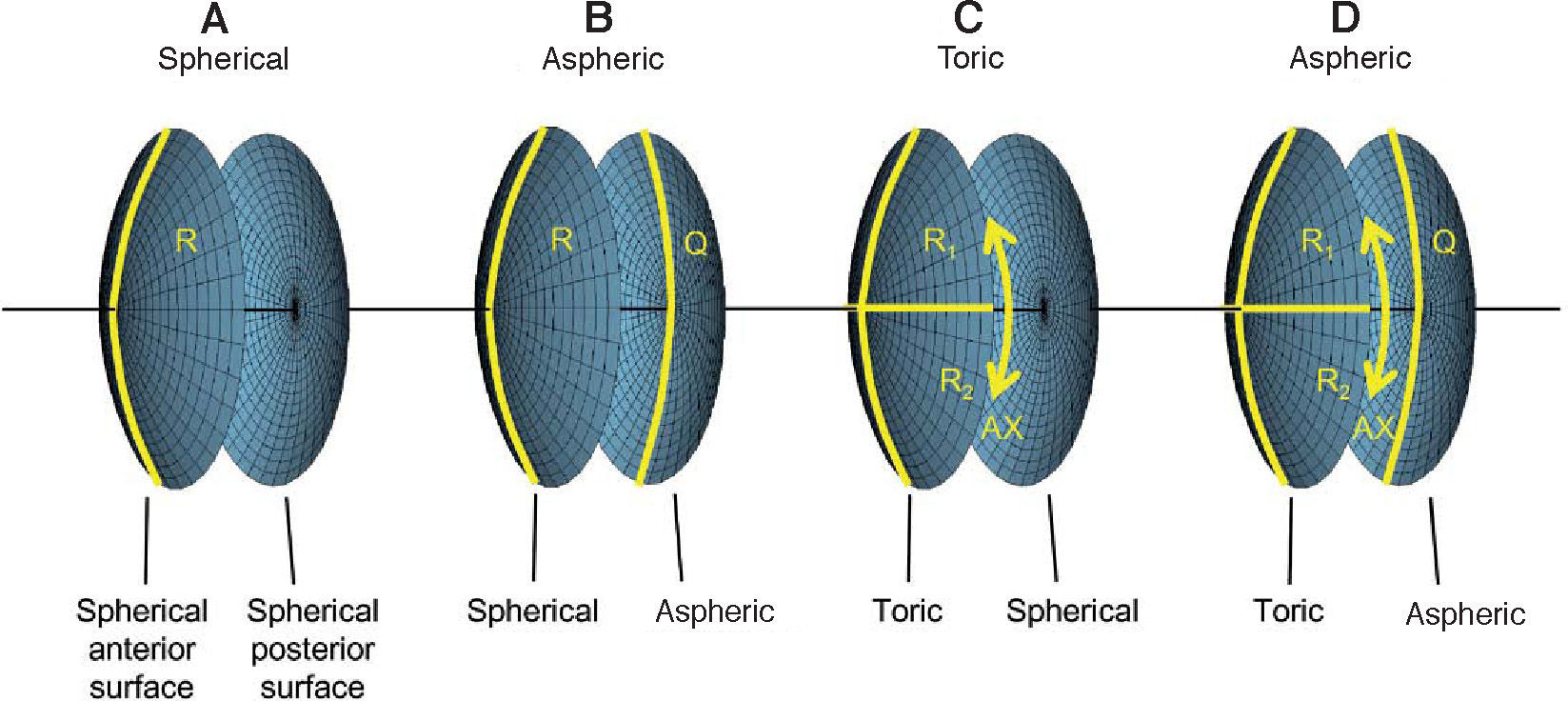
Types of customized IOLs. Depending on the complexity of the lens one or more parameters need to be calculated, resulting in a one- or a multi-dimensional optimization procedure. The degrees of freedom of the biconic anterior and posterior surfaces are shown for A. A spherical IOL, B. An aspheric IOL, C. A toric IOL and D. A toric aspheric IOL.
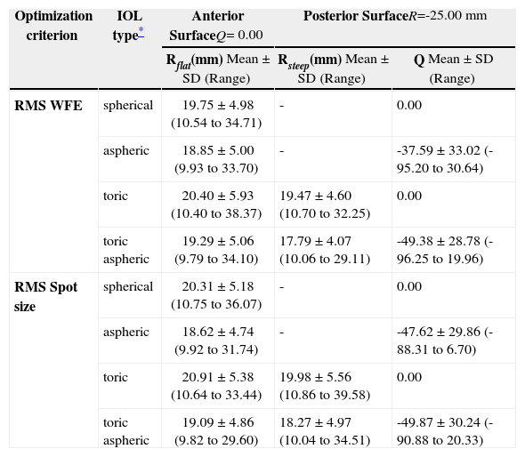
The radius of curvature of the posterior surface is held constant (Rpost = -25 mm). This is, of course, just one possible way to design toric aspheric IOLs. As optimization criteria both RMS WFE and RMS spot size are used. For the assessment of the optical properties, the residual wavefront aberration relative to the videokeratometric axis59 [p. 30 ff.] is calculated and approximated by Zernike polynomials. A pupil diameter of 6mm is assumed for the calculation of the IOLs as well as for the wavefront analysis.
ResultsThe diagrams in figure 8 show the Zernike analysis of the wavefronts. Even though Zernike polynomials up to the 6th order (28 terms) were fitted to the wavefront, only those Zernike modes up to the 4th order are shown for the sake of simplicity (thus omitting 13 terms, including the Z(6,0) coefficient) without hiding important information, because the 5th- and 6th-order coefficients are rather small. The zeroand first-order terms, piston and tilt, are not shown either; piston is only a constant offset without further relevance. Tilt causes a displacement of the image with respect to the center of the fovea, which can likely be compensated by the eye by adjusting the fixation angle.66 Thus, the individual Zernike coefficients start in the 5th column, ranging from astigmatism to quadrafoil. All Zernike coefficients refer to RMS in microns, as they are calculated according to the standards of the Optical society of America.67 The left four columns give RMS error values representing combined Zernike modes: total RMS gives the total RMS error (excluding piston and tilt), LOA RMS combines 2nd-order (lower order) aberrations (astigmatism and defocus), HOA RMS combines 3rd- to 6th-order (higher order) aberrations, SA RMS combines primary spherical aberration Z(4,0) and secondary spherical aberration Z(6,0). Note that, per definition, the individual Zernike coefficients are relative and do have a numerical sign, while the combined RMS values are absolute and are thus always positive. When interpreting the diagrams we bear the reader to keep also in mind that the combined RMS errors can be calculated directly from the individual Zernike coefficients as the square root of the sum of the squared coefficients, e.g.68

Figure 8A shows the residual wavefront aberration when optimized for RMS WFE. The bars and numbers indicate mean values, while the error bars specify the standard deviation. The mean defocus is around zero for all types of IOLs and the standard deviation is small. The big standard deviation corresponding to astigmatism is almost completely eliminated by the toric IOLs; this can also be seen when looking at the LOA RMS. The SA RMS is reduced both with the aspheric and with the toric aspheric IOLs, but not completely to zero. Figure 8B shows the results of the optimization for the same eyes but when taking RMS spot size as criterion.
These are very similar for the aspheric and the toric aspheric IOLs, but there are some differences for the spherical and the toric IOLs: in the presence of spherical aberration, the RMS spot size seems to be smaller when there is some amount of defocus left.
Table 2 shows the geometries of the different calculated IOLs. When comparing spherical and aspheric IOLs, the following interrelation can be observed: when some asphericity is added to the posterior surface, the radius of curvature of the anterior surface needs to be changed, too. The asphericities of the posterior surface for the IOLs are mainly hyperbolic; a big standard deviation is observed.
Geometries of the IOLs calculated
| Optimization criterion | IOL type* | Anterior SurfaceQ= 0.00 | Posterior SurfaceR=-25.00 mm | |
| Rflat(mm) Mean ± SD (Range) | Rsteep(mm) Mean ± SD (Range) | Q Mean ± SD (Range) | ||
| RMS WFE | spherical | 19.75 ± 4.98 (10.54 to 34.71) | - | 0.00 |
| aspheric | 18.85 ± 5.00 (9.93 to 33.70) | - | -37.59 ± 33.02 (-95.20 to 30.64) | |
| toric | 20.40 ± 5.93 (10.40 to 38.37) | 19.47 ± 4.60 (10.70 to 32.25) | 0.00 | |
| toric aspheric | 19.29 ± 5.06 (9.79 to 34.10) | 17.79 ± 4.07 (10.06 to 29.11) | -49.38 ± 28.78 (-96.25 to 19.96) | |
| RMS Spot size | spherical | 20.31 ± 5.18 (10.75 to 36.07) | - | 0.00 |
| aspheric | 18.62 ± 4.74 (9.92 to 31.74) | - | -47.62 ± 29.86 (-88.31 to 6.70) | |
| toric | 20.91 ± 5.38 (10.64 to 33.44) | 19.98 ± 5.56 (10.86 to 39.58) | 0.00 | |
| toric aspheric | 19.09 ± 4.86 (9.82 to 29.60) | 18.27 ± 4.97 (10.04 to 34.51) | -49.87 ± 30.24 (-90.88 to 20.33) | |
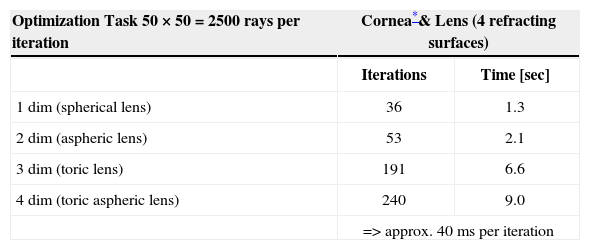
The calculation time is highly dependent on the starting conditions, the number of rays traced, the number of refracting surfaces and the number of variables in the optimization process. Table 3 shows the typical number of iterations and calculation time for the optimization tasks in this study. The ray-tracing program was developed in the C++ programming language, using Microsoft Visual Studio .NET 2003 and Microsoft Windows XP (Microsoft Corporation, USA) as operating system. All calculations were performed with a standard personal computer equipped with an Intel Pentium 4 2.6 GHz processor (Intel Corporation, USA).
Calculation time for optimization tasks
| Optimization Task 50 × 50 = 2500 rays per iteration | Cornea*& Lens (4 refracting surfaces) | |
| Iterations | Time [sec] | |
| 1 dim (spherical lens) | 36 | 1.3 |
| 2 dim (aspheric lens) | 53 | 2.1 |
| 3 dim (toric lens) | 191 | 6.6 |
| 4 dim (toric aspheric lens) | 240 | 9.0 |
| => approx. 40 ms per iteration | ||
The individual virtual eye combines two scientific fields: computer science and medicine. Computer science provides the computer technical structures and methods for the realization of a virtual eye to allow for simulation regarding the optical properties and, furthermore, to allow for the calculation of its optical components. This leads to contributions to medicine, as there are clinically relevant ophthalmological applications of this computer model.
The optical components of the virtual eye are modeled by means of mathematical surfaces that are feasible in terms of physiology and optical properties, as well as efficiently usable for computational ray tracing. The virtual cornea is modeled by applying a spline-based interpolation schema to the corneal elevation data of individual patients obtained experimentally in polar coordinate form, preferably from a Placido videotopometer. The interpolation schema enables the calculation of corneal elevation data and surface normal at any generic position. This leads to the possibility to do a ray tracing of uniformly distributed rays through the virtual eye. The implementation of this interpolation schema requires some time-consuming operations, such as the functional spline interpolation, to be performed only once in a preprocessing step, while the ray-surface intersection calculations don’t use expensive (time-consuming) routines. This efficient implementation makes the virtual cornea usable in conjunction with numerical methods for finding ray-surface intersections. The virtual lens is modeled by means of two biconic surfaces. Surface elevation and normals can be evaluated efficiently at any position algebraically. This modeling represents only a rough approximation to a human crystalline lens, which has a non-homogeneous gradient index69 – however most kinds of artificial lenses can be specified this way, including toric and aspheric lenses.
The optical properties of the virtual eye are simulated with RRT. Since the components were modeled particularly with regard to ray-surface intersection and surface normal calculations, many real rays can be traced through the virtual eye efficiently using numerical methods. Snell's law is used at every refracting surface and geometric optic criteria for the assessment of optical quality can be calculated: RMS spot size and wavefront aberration, both common metrics in technical optics. The wavefront aberration can be specified either as a combined RMS wavefront error or, alternatively, Zernike polynomials can be used for approximation to allow for a more detailed analysis of the kind of residual optical error.
Beyond only simulating optics, optical components can also be calculated by formulating and solving an optimization problem. The input of such an optimization problem can be the geometry of an IOL, as shown in this study. Depending on the type of lens, one or more input parameters are possible. The output criterion to be minimized can be either the RMS spot size of the RMS wavefront error. This optimization process is solved by means of numerical methods, resulting in an iterative minimization procedure either in one or in multiple dimensions.
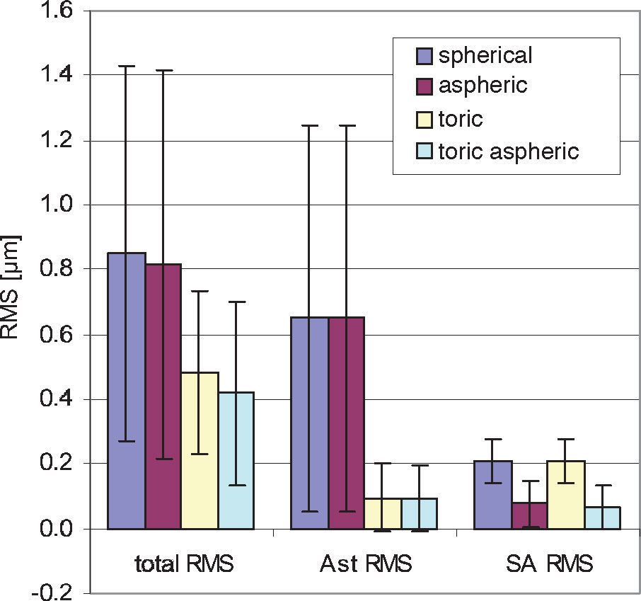
One application of the individual virtual eye is IOL calculation for cataract surgery. In a previous work it was shown that RRT – used to calculate basic spherical IOLs – is able to compete with current IOL calculation formulae for normal eyes. Unlike those IOL calculation formulae currently used that rely on paraxial optics and corneal keratometry readings, the calculation of IOLs with RRT accounts for a potentially irregular corneal topography (including HOAs) and, therefore, has the potential to overcome certain limitations of current calculation methods, like lens calculation after refractive surgery.58 The ray-tracing and optimization methods used in the previous study are identical to the ones described in more detail in the present paper. The optimization necessary for the spherical IOLs consisted of a one-dimensional minimization procedure. The present paper moves one step further and shows that even more advanced IOL geometries can be calculated with the individual virtual eye, resulting in a multi-dimensional optimization. Such a calculation of IOLs of complex shape for an individual patient cannot be attained with the formulae that are currently used. The residual wavefront aberration for the different kinds of IOLs was finally analyzed by means of Zernike polynomials. Furthermore, as optimizing criterion both the RMS spot size and the RMS WFE was used. A difference in the resulting IOL geometry was found depending on the criterion of choice– so minimizing RMS WFE or minimizing RMS spot size is generally not the same. When choosing RMS spot size the results of all calculations show that there is some interaction between spherical aberration and defocus (Figure 8): when there is some positive SA RMS left, optimizing spot size leads to negative defocus, while optimizing WFE guarantees almost zero defocus. However, when aspheric IOLs are calculated, there tend to be only minor differences between optimizing RMS WFE and optimizing RMS spot size. Apart from the effect of choosing one optimization criterion or the other, the impact of the type of IOL on the residual wavefront aberration can be nicely seen by analyzing the Zernike polynomials. Figure 9 summarizes the most relevant combined Zernike modes from figure 8A: The more complex the IOL calculated is, the lower is the total wavefront error (Figure 9, left bars). The spherical IOL is only able to correct for the defocus, while toric IOLs also eliminate astigmatism (Figure 9, middle bars). The spherical aberration is additionally reduced with the aspheric and the toric aspheric IOLs (Figure 9, right bars).
 and the aspherical component (SA RMS) reducing spherical aberration.")
Summarized wavefront aberration with different IOL types for minimized RMS WFE. As the complexity of the IOL increases, the residual total wavefront error decreases. This is the result of the toric component reducing astigmatism (Ast RMS) and the aspherical component (SA RMS) reducing spherical aberration.
Although these simulated results of the residual wavefront aberration using individual patient data are theoretical so far, relevant implications may already be derived for clinical practice. The astigmatism of a pseudophakic eye can be corrected by either manipulating the shape of the cornea itself with incisional corneal relaxing techniques or with laser ablation or –without changing the cornea– by means of spectacles, contact lenses or toric IOLs.70 In this study the astigmatism was corrected with the toric surface of the IOL – but can principally be corrected just as well by means of spectacles without being affected by the asphericity of the lens and its resulting impact on the spherical aberration. The use of aspheric IOLs is being discussed extensively in literature. A conventional IOL with spherical surfaces has positive spherical aberration, which amplifies the average positive corneal spherical aberration of a patient. To avoid this, clinical practice is to use aspheric IOLs with a fixed amount of zero or negative spherical aberration, intended to compensate to a certain degree the average positive corneal spherical aberration.28 In contrast to this approach and as a more advanced one, the aspheric IOLs calculated in this study are customized, meaning that the asphericity of the IOL is calculated for each patient individually. The resulting wavefront analysis shows that the spherical aberration of the eye is reduced, even though total HOAs are still large according to the theoretical prediction, so the potential benefit in terms of visual performance may be limited, even with customized aspheric IOLs. The wavefront aberration calculated in this study can be compared to actual measurements of pseudophakic patients, for example those obtained with a Hartmann-Shack wavefront sensor. As a contribution to the controversial discussion about the benefits of aspheric IOLs,71 such a comparison and a discussion of the clinical implications will be presented in a separate investigation since it is beyond the more technical scope of this paper.
Which criterion the human eye actually uses for focusing is unknown.59 [p. 152] Both, the RMS WFE and RMS spot size are metrics used in technical optics. Visual performance metrics, such as visual acuity or contrast sensitivity, can not be generally assessed from geometrical optical quantities alone, since there are also other physiological factors involved, from the retina and the brain. Even though Applegate et al. found a significant correlation between RMS WFE and visual performance,72 – in a later study they confined their findings to relatively high levels of aberration, and concluded that the RMS WFE is not a good predictor of visual acuity for low levels of aberration.73 Other studies have also shown that different kinds of aberrations interact with each other74 and that they are not all equally important regarding their impact on visual performance.75,76 For a future extension of the virtual eye model, regarding issues beyond geometrical optics, it might be very interesting to incorporate the results of recent investigations studying the relation between wavefront aberration and visual performance.77-81
The accuracy of RRT is directly affected by the input data from measurements of the patient eyes – so it will directly benefit from improvements in the measurement devices, especially regarding corneal elevation. It will also benefit from the inclusion of measured geometry that is currently not assessed in most cases in clinical practice, such as the posterior corneal surface. Currently, measurements from different devices are used to construct the individual virtual eye (like those from a videokeratometer and a those from a PCI device to measure axial length). Once possible – maybe thanks to the combination of different measuring methods – it would be desirable to have one single measurement device that completely measured the geometry of the whole eye including cornea, lens and segmental lengths. Since the calculations performed in this study might also be done with other ray-tracing programs, the focus of this computer model lies in the development of a specifically designed standalone program. High value was placed on obtaining an efficient implementation of the time-critical numerical ray-tracing and optimization procedures, leading to short calculation times. This eye model could be integrated in such a combined measuring device, capturing the whole eye and leading to practicable methods, especially for IOL calculation. Moreover, the effects of misalignment of IOLs could be assessed, like tilt and decentration. Further application fields also include phakic IOLs, ablation profiles for corneal refractive laser surgery or combined surgical procedures. One major remaining challenge, in order to be able to extend the capabilities and, therefore, the potential applications of the individual virtual eye, is the proper simulation of the human crystalline lens. Another challenge is the further development trying to attain a more realistic model, by incorporating polychromatic issues or additional physical properties beyond geometrical optics, like diffraction and scattering. Finally, there is a wide scope when extending the individual virtual eye by addressing those issues beyond optics regarding physiology of the retina and brain.
The author would like to thank the Dr. Ernst und Wilma-Müller-Stiftung, Stuttgart, Germany, for their financial support and Ainura Stanbekova for acquiring the clinical data.
Commercial variants based on this as VOL-Pro and VOL-CT (former CTView) are sold by Sarver and Associates, Inc. (USA; http://saavision.com).


